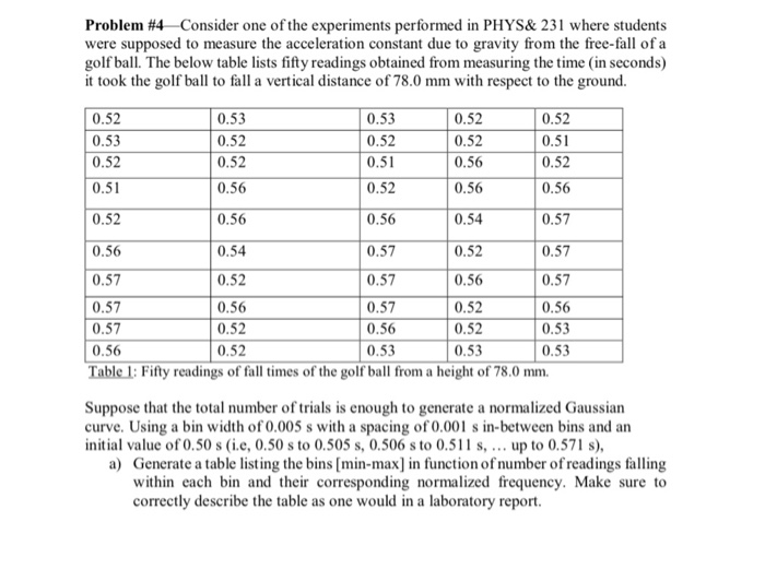
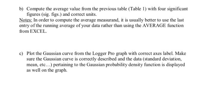
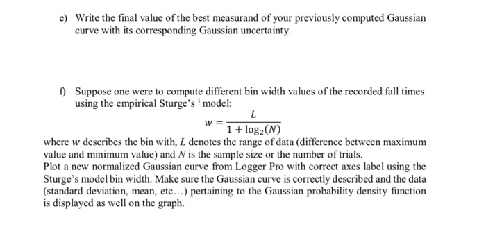
Problem #4 Consider one of the experiments performed in PHYS& 231 where students were supposed to measure the acceleration constant due to gravity from the free-fall of a golf ball. The below table lists fifty readings obtained from measuring the time (in seconds) it took the golf ball to fall a vertical distance of 78.0 mm with respect to the ground. 0.52 0.53 0.52 0.51 0.52 0.53 0.52 0.52 0.56 0.53 0.52 0.51 0.52 0.52 0.52 0.56 0.56 0.54 0.52 0.51 0.52 0.56 0.56 0.56 0.57 0.56 0.54 0.57 0.52 0.57 0.57 0.52 0.57 0.56 0.57 0.57 0.56 0.57 0.52 0.56 0.57 0.52 0.56 0.52 0.53 0.56 0.52 0.53 0.53 0.53 Table 1: Fifty readings of fall times of the golf ball from a height of 78.0 mm. Suppose that the total number of trials is enough to generate a normalized Gaussian curve. Using a bin width of 0.005s with a spacing of 0.001 s in-between bins and an initial value of 0.50 s (i.e, 0.50 s to 0.505 s, 0.506 s to 0.511 s, ... up to 0.571 s), a) Generate a table listing the bins (min-max) in function of number of readings falling within each bin and their corresponding normalized frequency. Make sure to correctly describe the table as one would in a laboratory report. b) Compute the average value from the previous table (Table 1) with four significant figures (sig. figs.) and correct units. Notes: In order to compute the average measurand, it is usually better to use the last entry of the running average of your data rather than using the AVERAGE function from EXCEL c) Plot the Gaussian curve from the Logger Pro graph with correct axes label. Make sure the Gaussian curve is correctly described and the data (standard deviation, mean, etc...) pertaining to the Gaussian probability density function is displayed as well on the graph. d) Determine the variance, standard deviation and uncertainty of your above Gaussian using four sig. figs. e) Write the final value of the best measurand of your previously computed Gaussian curve with its corresponding Gaussian uncertainty. f) Suppose one were to compute different bin width values of the recorded fall times using the empirical Sturge's ' model: L w 1 + log (N) where w describes the bin with, L denotes the range of data (difference between maximum value and minimum value) and N is the sample size or the number of trials. Plot a new normalized Gaussian curve from Logger Pro with correct axes label using the Sturge's model bin width. Make sure the Gaussian curve is correctly described and the data (standard deviation, mean, etc...) pertaining to the Gaussian probability density function is displayed as well on the graph. g) Compute the standard deviation and uncertainty of the data (using four sig. figs) from Table 1 using Type A: Discrete PDF. h) By comparing the measurand values of the previously plotted Gaussian PDFs to the ones obtained from Type A Discrete, argue which Gaussian PDF generates more accurate values of the mean and uncertainty of the fall times. Problem #4 Consider one of the experiments performed in PHYS& 231 where students were supposed to measure the acceleration constant due to gravity from the free-fall of a golf ball. The below table lists fifty readings obtained from measuring the time (in seconds) it took the golf ball to fall a vertical distance of 78.0 mm with respect to the ground. 0.52 0.53 0.52 0.51 0.52 0.53 0.52 0.52 0.56 0.53 0.52 0.51 0.52 0.52 0.52 0.56 0.56 0.54 0.52 0.51 0.52 0.56 0.56 0.56 0.57 0.56 0.54 0.57 0.52 0.57 0.57 0.52 0.57 0.56 0.57 0.57 0.56 0.57 0.52 0.56 0.57 0.52 0.56 0.52 0.53 0.56 0.52 0.53 0.53 0.53 Table 1: Fifty readings of fall times of the golf ball from a height of 78.0 mm. Suppose that the total number of trials is enough to generate a normalized Gaussian curve. Using a bin width of 0.005s with a spacing of 0.001 s in-between bins and an initial value of 0.50 s (i.e, 0.50 s to 0.505 s, 0.506 s to 0.511 s, ... up to 0.571 s), a) Generate a table listing the bins (min-max) in function of number of readings falling within each bin and their corresponding normalized frequency. Make sure to correctly describe the table as one would in a laboratory report. b) Compute the average value from the previous table (Table 1) with four significant figures (sig. figs.) and correct units. Notes: In order to compute the average measurand, it is usually better to use the last entry of the running average of your data rather than using the AVERAGE function from EXCEL c) Plot the Gaussian curve from the Logger Pro graph with correct axes label. Make sure the Gaussian curve is correctly described and the data (standard deviation, mean, etc...) pertaining to the Gaussian probability density function is displayed as well on the graph. d) Determine the variance, standard deviation and uncertainty of your above Gaussian using four sig. figs. e) Write the final value of the best measurand of your previously computed Gaussian curve with its corresponding Gaussian uncertainty. f) Suppose one were to compute different bin width values of the recorded fall times using the empirical Sturge's ' model: L w 1 + log (N) where w describes the bin with, L denotes the range of data (difference between maximum value and minimum value) and N is the sample size or the number of trials. Plot a new normalized Gaussian curve from Logger Pro with correct axes label using the Sturge's model bin width. Make sure the Gaussian curve is correctly described and the data (standard deviation, mean, etc...) pertaining to the Gaussian probability density function is displayed as well on the graph. g) Compute the standard deviation and uncertainty of the data (using four sig. figs) from Table 1 using Type A: Discrete PDF. h) By comparing the measurand values of the previously plotted Gaussian PDFs to the ones obtained from Type A Discrete, argue which Gaussian PDF generates more accurate values of the mean and uncertainty of the fall times