Question
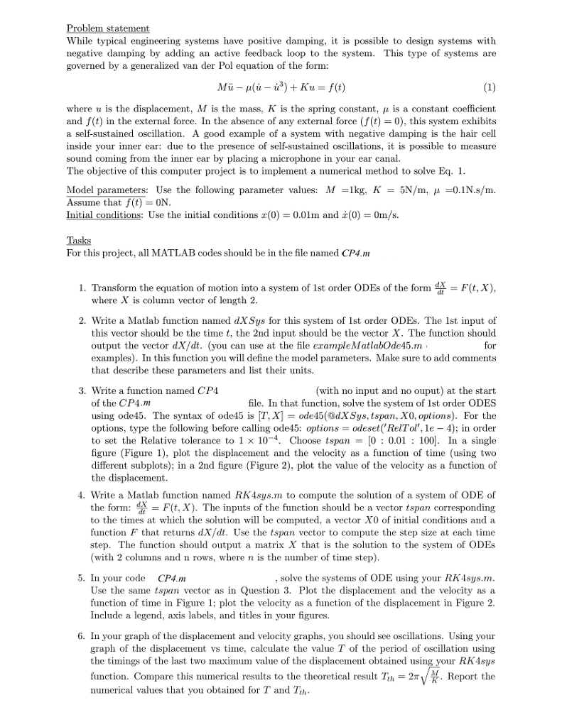
Problem statement While typical engineering systems have positive damping, it is possible to design systems with negative damping by adding an active feedback loop to
Problem statement While typical engineering systems have positive damping, it is possible to design systems with negative damping by adding an active feedback loop to the system. This type of systems are governed by a generalized van der Pol equation of the form:
Mu (u u 3) + Ku = f(t) (1)
where u is the displacement, M is the mass, K is the spring constant, is a constant coefficient and f(t) in the external force. In the absence of any external force (f(t) = 0), this system exhibits a self-sustained oscillation. A good example of a system with negative damping is the hair cell inside your inner ear: due to the presence of self-sustained oscillations, it is possible to measure sound coming from the inner ear by placing a microphone in your ear canal.
The objective of this computer project is to implement a numerical method to solve Eq. 1.
Model parameters: Use the following parameter values: M =1kg, K = 5N/m, =0.1N.s/m. Assume that f(t) = 0N. Initial conditions: Use the initial conditions x(0) = 0.01m and x (0) = 0m/s.
Tasks For this project, all MATLAB codes should be in the file named CP4.m where Lastname is your last name and Firstname is your first name.
Transform the equation of motion into a system of 1st order ODEs of the form dX = F (t, X ), dt
where X is column vector of length 2.
Write a Matlab function named dXSys for this system of 1st order ODEs. The 1st input of this vector should be the time t, the 2nd input should be the vector X. The function should output the vector dX/dt. (you can use at the file exampleMatlabOde45.m for examples). In this function you will define the model parameters. Make sure to add comments that describe these parameters and list their units.
Write a function named CP4 (with no input and no ouput) at the start of the CP4.m file. In that function, solve the system of 1st order ODES using ode45. The syntax of ode45 is [T,X] = ode45(@dXSys,tspan,X0,options). For the options, type the following before calling ode45: options = odeset(RelT ol, 1e 4); in order to set the Relative tolerance to 1 104. Choose tspan = [0 : 0.01 : 100]. In a single figure (Figure 1), plot the displacement and the velocity as a function of time (using two different subplots); in a 2nd figure (Figure 2), plot the value of the velocity as a function of the displacement.
1
Write a Matlab function named RK4sys.m to compute the solution of a system of ODE of the form: dX = F(t,X). The inputs of the function should be a vector tspan corresponding
dt
to the times at which the solution will be computed, a vector X0 of initial conditions and a function F that returns dX/dt. Use the tspan vector to compute the step size at each time step. The function should output a matrix X that is the solution to the system of ODEs (with 2 columns and n rows, where n is the number of time step).
In your code CP4.m, solve the systems of ODE using your RK4sys.m. Use the same tspan vector as in Question 3. Plot the displacement and the velocity as a function of time in Figure 1; plot the velocity as a function of the displacement in Figure 2. Include a legend, axis labels, and titles in your figures.
In your graph of the displacement and velocity graphs, you should see oscillations. Using your
graph of the displacement vs time, calculate the value T of the period of oscillation using
the timings of the last two maximum value of the displacement obtained using your RK4sys
function. Compare this numerical results to the theoretical result Tth = 2 numerical values that you obtained for T and Tth.
M . Report the K

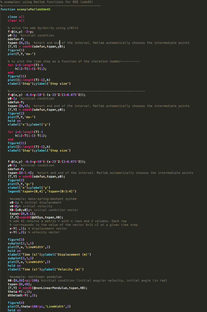
% examples: using Matlab functions for ODE (ode45) %----------------------------------------------------- function exampleMatlabOde45
close all clear all
% solve the ode dy/dx=-2y using y(0)=1 f=@(x,y) -2*y; y0=1; %initial condition odefun=f; tspan=[0,2]; %start and end of the interval. Matlab automatically chooses the intermediate points [T,Y] = ode45(odefun,tspan,y0); figure(1) plot(T,Y,'mx-')
% to plot the time step as a function of the iteration number---------- for i=1:length(T)-1 h(i)=T(i+1)-T(i); end figure(11) plot([1:length(T)-1],h) xlabel('Step');ylabel('Step size')
%------------------------------------------------------------------------- f=@(x,y) -0.6*y+10^(-(x-2)^2/(2*0.075^2)); y0=1; %initial condition odefun=f; tspan=[0,4]; %start and end of the interval. Matlab automatically chooses the intermediate points [T,Y] = ode45(odefun,tspan,y0); figure(2) plot(T,Y,'mx-') hold on xlabel('x');ylabel('y')
for i=1:length(T)-1 h(i)=T(i+1)-T(i); end figure(21) plot([1:length(T)-1],h) xlabel('Step');ylabel('Step size')
f=@(x,y) -0.6*y+10^(-(x-2)^2/(2*0.075^2)); y0=1; %initial condition odefun=f; tspan=[0:1:4]; %start and end of the interval. Matlab automatically chooses the intermediate points [T,Y] = ode45(odefun,tspan,y0); figure(2) plot(T,Y,'g-') xlabel('x');ylabel('y') legend('tspan=[0,4]','tspan=[0:1:4]')
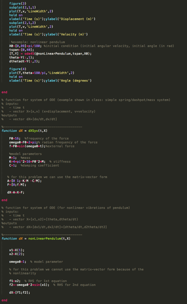
%example: mass-spring-dashpot system x0=1; % initial displacement v0=0;% initial velocity X0=[x0;v0];% initial condition vector tspan=[0,0.1]; [T,Y]=ode45(@dXSys,tspan,X0); % ode 45 returns a matrix Y with n rows and 2 columns. Each row % corresponds to the value of the vector X=[x v] at a given time step x=Y(:,1); % displacement vector v=Y(:,2); % velocity vector figure(3) subplot(2,1,1) plot(T,x,'LineWidth',2) hold on xlabel('Time (s)');ylabel('Displacement (m)') subplot(2,1,2) plot(T,v,'LineWidth',2) hold on xlabel('Time (s)');ylabel('Velocity (m)') %example: nonlinear pendulum X0=[0,89]*pi/180; %initial condition (initial angular velocity, initial angle (in rad) tspan=[0,40]; [T,Y] = ode45(@nonLinearPendulum,tspan,X0); theta=Y(:,1); dthetadt=Y(:,2);
figure(4) plot(T,theta*180/pi,'LineWidth',2) hold on xlabel('Time (s)');ylabel('Angle (degrees')
end
% function for system of ODE (example shown in class: simple spring/dashpot/mass system) % inputs: % - time t % - vector X=[x,v] (x=displacement, v=velocity) %outputs % - vector dX=[dx/dt,dv/dt]
%----------------------------------------- function dX = dXSys(t,X)
F0=16; %frequency of the force omega0=F0*2*pi;% radian frequency of the force f=F0*sin(omega0*t);%external force %model parameters M=1; %mass K=4*pi^2*16*F0^2*M; % stiffness C=1; %damping coefficient % for this problem we can use the matrix-vector form A=[0 1;-K/M -C/M]; F=[0;f/M]; dX=A*X+F; end
% function for system of ODE (for nonlinear vibrations of pendulum) % inputs: % - time t % - vector X=[x1,x2]=[theta,dtheta/dt) %outputs % - vector dX=[dx1/dt,dx2/dt]=[dtheta/dt,d2theta/dt2]
%----------------------------------------- function dX = nonLinearPendulum(t,X)
x1=X(1); x2=X(2);
omega0=1; % model parameter % for this problem we cannot use the matrix-vector form because of the % nonlinearity f1=x2; % RHS for 1st equation f2=-omega0^2*sin(x1); % RHS for 2nd equation dX=[f1;f2]; end


Step by Step Solution
There are 3 Steps involved in it
Step: 1

Get Instant Access to Expert-Tailored Solutions
See step-by-step solutions with expert insights and AI powered tools for academic success
Step: 2

Step: 3

Ace Your Homework with AI
Get the answers you need in no time with our AI-driven, step-by-step assistance
Get Started


