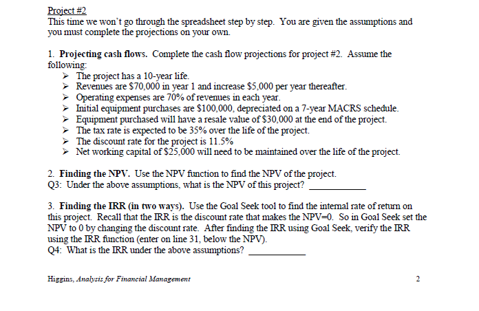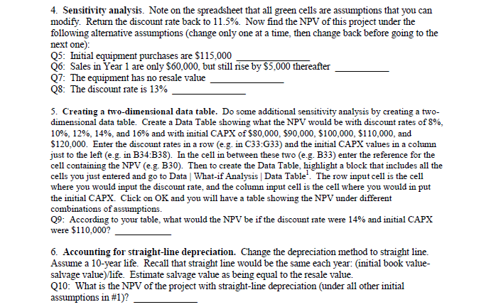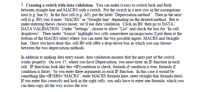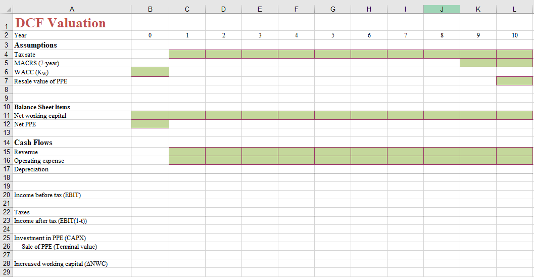
Project #2 This time we won't go through the spreadsheet step by step. You are given the assumptions and you must complete the projections on your own. 1. Projecting cash flows. Complete the cash flow projections for project #2. Assume the following: The project has a 10-year life. Revenues are $70,000 in year 1 and increase $5,000 per year thereafter. Operating expenses are 70% of revenues in each year. Initial equipment purchases are $100,000, depreciated on a 7-year MACRS schedule. Equipment purchased will have a resale value of $30,000 at the end of the project. The tax rate is expected to be 35% over the life of the project. The discount rate for the project is 11.5% Net working capital of $25,000 will need to be maintained over the life of the project. 2. Finding the NPV. Use the NPV function to find the NPV of the project. Q3: Under the above assumptions, what is the NPV of this project? 3. Finding the IRR (in two ways). Use the Goal Seek tool to find the internal rate of return on this project. Recall that the IRR is the discount rate that makes the NPV=O. So in Goal Seek set the NPV to O by changing the discount rate. After finding the IRR using Goal Seek, verify the RR using the IRR function (enter on line 31, below the NPV). 04: What is the IRR under the above assumptions? Higgins, Analysis for Financial Management 2 4. Sensitivity analysis. Note on the spreadsheet that all green cells are assumptions that you can modify. Return the discount rate back to 11.5%. Now find the NPV of this project under the following alternative assumptions (change only one at a time, then change back before going to the next one): Q5: Initial equipment purchases are $115,000 Q6: Sales in Year 1 are only $60,000, but still rise by $5,000 thereafter 07: The equipment has no resale value 08: The discount rate is 13% 5. Creating a two-dimensional data table. Do some additional sensitivity analysis by creating a two- dimensional data table. Create a Data Table showing what the NPV would be with discount rates of 8%, 10%, 12%, 14%, and 16% and with initial CAPX of $80,000 $90,000, $100,000, $110,000, and $120,000. Enter the discount rates in a row (e.g. in C33:G33) and the initial CAPX values in a column just to the left (e.g. in B34:B38). In the cell in between these two (e.g. B33) enter the reference for the cell containing the NPV (e.g. B30). Then to create the Data Table highlight a block that includes all the cells you just entered and go to Data | What-if Analysis | Data Table? The row input cell is the cell where you would input the discount rate, and the column input cell is the cell where you would in put the initial CAPX. Click on OK and you will have a table showing the NPV under different combinations of assumptions. Q9: According to your table, what would the NPV be if the discount rate were 14% and initial CAPX were $110,000? 6. Accounting for straight-line depreciation. Change the depreciation method to straight line. Assume a 10-year life. Recall that straight line would be the same each year: initial book value- salvage value)/life. Estimate salvage value as being equal to the resale value. Q10: What is the NPV of the project with straight-line depreciation (under all other initial assumptions in #1)? 7. Creating a switch with data validation. You can make it easy to switch back and forth between straight-line and MACRS with a switch. Put the switch in a new row in the assumptions area (eg. line 9). In the first cell (eg. A9), put the label "Depreciation method. Then in the next cell (eg. B9) you'd enter "MACRS" or "Straight-line" depending on the desired method. But to make entering theses choice easier, we'll use data validation Click on B9, then go to DATA DATA VALDATION. Under "Settings, choose to allow List and check the box for In-cell dropdown. Then under "Source highlight two cells somewhere inconspicuous (I put them at the bottom of the MACRS table) where you can enter the two possible inputs: MACRS and Straight- line. Once you have done this, cell B9 will offer a drop-down box in which you can choose between the two depreciation methods. In addition to making data entry easier, data validation ensures that the next part of the switch works properly. On row 17, where you have Depreciation, you must enter an IF function in each cell. IF functions look like this =IF (condition to check formula if condition is true, formula if condition is false). So you enter three arguments in each IF function. In this case it would be something like = F($B9="MACRS, enter MACRS formula here, enter straight-line formula here). If you enter this correctly and lock in the right cells, you only have to enter one formula, which you can then copy all the way across the row. B D E F G H J K L 0 1 2 3 4 5 6 7 8 9 10 DCF Valuation 1 2 Year 3 Assumptions 4 Tax rate 5 MACRS (7-year) 6 WACC (Kw) 7 Resale value of PPE 8 9 10 Balance Sheet Items 11 Net working capital 12 Net PPE 13 14 Cash Flows 15 Revenue 16 Operating expense 17 Depreciation 18 19 20 Income before tax (EBIT) 21 22 Taxes 23 Income after tax (EBIT(1-t)) 24 25 Investment in PPE (CAPX) 26 Sale of PPE (Terminal value) 27 28 Increased working capital (ANWC) 29 Project #2 This time we won't go through the spreadsheet step by step. You are given the assumptions and you must complete the projections on your own. 1. Projecting cash flows. Complete the cash flow projections for project #2. Assume the following: The project has a 10-year life. Revenues are $70,000 in year 1 and increase $5,000 per year thereafter. Operating expenses are 70% of revenues in each year. Initial equipment purchases are $100,000, depreciated on a 7-year MACRS schedule. Equipment purchased will have a resale value of $30,000 at the end of the project. The tax rate is expected to be 35% over the life of the project. The discount rate for the project is 11.5% Net working capital of $25,000 will need to be maintained over the life of the project. 2. Finding the NPV. Use the NPV function to find the NPV of the project. Q3: Under the above assumptions, what is the NPV of this project? 3. Finding the IRR (in two ways). Use the Goal Seek tool to find the internal rate of return on this project. Recall that the IRR is the discount rate that makes the NPV=O. So in Goal Seek set the NPV to O by changing the discount rate. After finding the IRR using Goal Seek, verify the RR using the IRR function (enter on line 31, below the NPV). 04: What is the IRR under the above assumptions? Higgins, Analysis for Financial Management 2 4. Sensitivity analysis. Note on the spreadsheet that all green cells are assumptions that you can modify. Return the discount rate back to 11.5%. Now find the NPV of this project under the following alternative assumptions (change only one at a time, then change back before going to the next one): Q5: Initial equipment purchases are $115,000 Q6: Sales in Year 1 are only $60,000, but still rise by $5,000 thereafter 07: The equipment has no resale value 08: The discount rate is 13% 5. Creating a two-dimensional data table. Do some additional sensitivity analysis by creating a two- dimensional data table. Create a Data Table showing what the NPV would be with discount rates of 8%, 10%, 12%, 14%, and 16% and with initial CAPX of $80,000 $90,000, $100,000, $110,000, and $120,000. Enter the discount rates in a row (e.g. in C33:G33) and the initial CAPX values in a column just to the left (e.g. in B34:B38). In the cell in between these two (e.g. B33) enter the reference for the cell containing the NPV (e.g. B30). Then to create the Data Table highlight a block that includes all the cells you just entered and go to Data | What-if Analysis | Data Table? The row input cell is the cell where you would input the discount rate, and the column input cell is the cell where you would in put the initial CAPX. Click on OK and you will have a table showing the NPV under different combinations of assumptions. Q9: According to your table, what would the NPV be if the discount rate were 14% and initial CAPX were $110,000? 6. Accounting for straight-line depreciation. Change the depreciation method to straight line. Assume a 10-year life. Recall that straight line would be the same each year: initial book value- salvage value)/life. Estimate salvage value as being equal to the resale value. Q10: What is the NPV of the project with straight-line depreciation (under all other initial assumptions in #1)? 7. Creating a switch with data validation. You can make it easy to switch back and forth between straight-line and MACRS with a switch. Put the switch in a new row in the assumptions area (eg. line 9). In the first cell (eg. A9), put the label "Depreciation method. Then in the next cell (eg. B9) you'd enter "MACRS" or "Straight-line" depending on the desired method. But to make entering theses choice easier, we'll use data validation Click on B9, then go to DATA DATA VALDATION. Under "Settings, choose to allow List and check the box for In-cell dropdown. Then under "Source highlight two cells somewhere inconspicuous (I put them at the bottom of the MACRS table) where you can enter the two possible inputs: MACRS and Straight- line. Once you have done this, cell B9 will offer a drop-down box in which you can choose between the two depreciation methods. In addition to making data entry easier, data validation ensures that the next part of the switch works properly. On row 17, where you have Depreciation, you must enter an IF function in each cell. IF functions look like this =IF (condition to check formula if condition is true, formula if condition is false). So you enter three arguments in each IF function. In this case it would be something like = F($B9="MACRS, enter MACRS formula here, enter straight-line formula here). If you enter this correctly and lock in the right cells, you only have to enter one formula, which you can then copy all the way across the row. B D E F G H J K L 0 1 2 3 4 5 6 7 8 9 10 DCF Valuation 1 2 Year 3 Assumptions 4 Tax rate 5 MACRS (7-year) 6 WACC (Kw) 7 Resale value of PPE 8 9 10 Balance Sheet Items 11 Net working capital 12 Net PPE 13 14 Cash Flows 15 Revenue 16 Operating expense 17 Depreciation 18 19 20 Income before tax (EBIT) 21 22 Taxes 23 Income after tax (EBIT(1-t)) 24 25 Investment in PPE (CAPX) 26 Sale of PPE (Terminal value) 27 28 Increased working capital (ANWC) 29