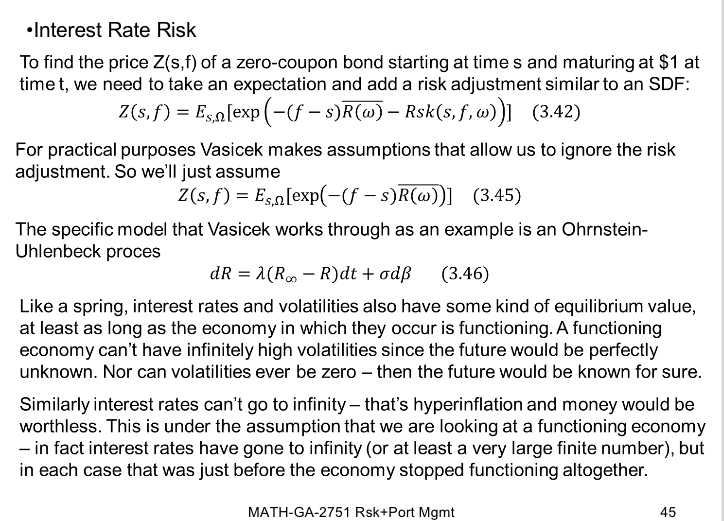
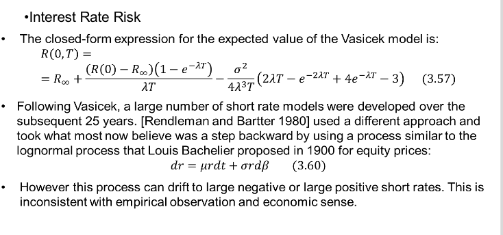
Prove that the expected long rate r(0,T) (as T gets large) will go negative in the Vasicek model as 0. In other words if there is no tension in the spring pulling it back to a long-term average,
an impossible situation will result. Use (3.57).


Interest Rate Risk To find the price Z(s,f) of a zero-coupon bond starting at times and maturing at $1 at time t, we need to take an expectation and add a risk adjustment similar to an SDF: Z(s,f) = Es,n[exp(-(f s)R(W) Rsk(s,f,w))) (3.42) For practical purposes Vasicek makes assumptions that allow us to ignore the risk adjustment. So we'll just assume Z(s,f) = Eso (exp(-(f -s)R(W))) (3.45) The specific model that Vasicek works through as an example is an Ohrnstein- Uhlenbeck proces dR = 1(RO - R)dt + odp (3.46) Like a spring, interest rates and volatilities also have some kind of equilibrium value, at least as long as the economy in which they occur is functioning. A functioning economy can't have infinitely high volatilities since the future would be perfectly unknown. Nor can volatilities ever be zero then the future would be known for sure. Similarly interest rates can't go to infinity - that's hyperinflation and money would be worthless. This is under the assumption that we are looking at a functioning economy - in fact interest rates have gone to infinity (or at least a very large finite number), but in each case that was just before the economy stopped functioning altogether. MATH-GA-2751 Rsk+Port Mgmt Interest Rate Risk The closed-form expression for the expected value of the Vasicek model is: R(0,T) = (R(0) - RO)(1-e-A7) 02 R + w(227-e-217 + 4e-17 3) (3.57) 27 42314 Following Vasicek, a large number of short rate models were developed over the subsequent 25 years. (Rendleman and Bartter 1980] used a different approach and took what most now believe was a step backward by using a process similar to the lognormal process that Louis Bachelier proposed in 1900 for equity prices: dr = urdt + ordB (3.60) However this process can drift to large negative or large positive short rates. This is inconsistent with empirical observation and economic sense. Interest Rate Risk The closed-form expression for the expected value of the Vasicek model is: R(0,T) = (R(0) - RO)(1-e-A7) 02 R + w(227-e-217 + 4e-17 3) (3.57) 27 42314 Following Vasicek, a large number of short rate models were developed over the subsequent 25 years. (Rendleman and Bartter 1980] used a different approach and took what most now believe was a step backward by using a process similar to the lognormal process that Louis Bachelier proposed in 1900 for equity prices: dr = urdt + ordB (3.60) However this process can drift to large negative or large positive short rates. This is inconsistent with empirical observation and economic sense. Interest Rate Risk To find the price Z(s,f) of a zero-coupon bond starting at times and maturing at $1 at time t, we need to take an expectation and add a risk adjustment similar to an SDF: Z(s,f) = Es,n[exp(-(f s)R(W) Rsk(s,f,w))) (3.42) For practical purposes Vasicek makes assumptions that allow us to ignore the risk adjustment. So we'll just assume Z(s,f) = Eso (exp(-(f -s)R(W))) (3.45) The specific model that Vasicek works through as an example is an Ohrnstein- Uhlenbeck proces dR = 1(RO - R)dt + odp (3.46) Like a spring, interest rates and volatilities also have some kind of equilibrium value, at least as long as the economy in which they occur is functioning. A functioning economy can't have infinitely high volatilities since the future would be perfectly unknown. Nor can volatilities ever be zero then the future would be known for sure. Similarly interest rates can't go to infinity - that's hyperinflation and money would be worthless. This is under the assumption that we are looking at a functioning economy - in fact interest rates have gone to infinity (or at least a very large finite number), but in each case that was just before the economy stopped functioning altogether. MATH-GA-2751 Rsk+Port Mgmt Interest Rate Risk The closed-form expression for the expected value of the Vasicek model is: R(0,T) = (R(0) - RO)(1-e-A7) 02 R + w(227-e-217 + 4e-17 3) (3.57) 27 42314 Following Vasicek, a large number of short rate models were developed over the subsequent 25 years. (Rendleman and Bartter 1980] used a different approach and took what most now believe was a step backward by using a process similar to the lognormal process that Louis Bachelier proposed in 1900 for equity prices: dr = urdt + ordB (3.60) However this process can drift to large negative or large positive short rates. This is inconsistent with empirical observation and economic sense. Interest Rate Risk The closed-form expression for the expected value of the Vasicek model is: R(0,T) = (R(0) - RO)(1-e-A7) 02 R + w(227-e-217 + 4e-17 3) (3.57) 27 42314 Following Vasicek, a large number of short rate models were developed over the subsequent 25 years. (Rendleman and Bartter 1980] used a different approach and took what most now believe was a step backward by using a process similar to the lognormal process that Louis Bachelier proposed in 1900 for equity prices: dr = urdt + ordB (3.60) However this process can drift to large negative or large positive short rates. This is inconsistent with empirical observation and economic sense
