Provide a summary technical report with about Pipelined Execution which is also named as Instruction Level Parallelism, addressing mainly the following areas: 1. What is Pipelined Execution and its purpose, 2. How it is implemented, 3. What are the major problems (hazards) of pipelined executions and common solution methods utilized to resolve these problems. - Add an extra section to the end of your report which puts emphasis on the differences among multithreading, multicore processors, and multiprocessing.

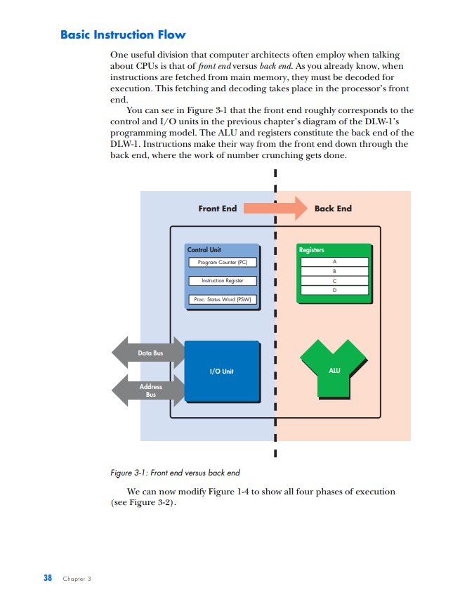
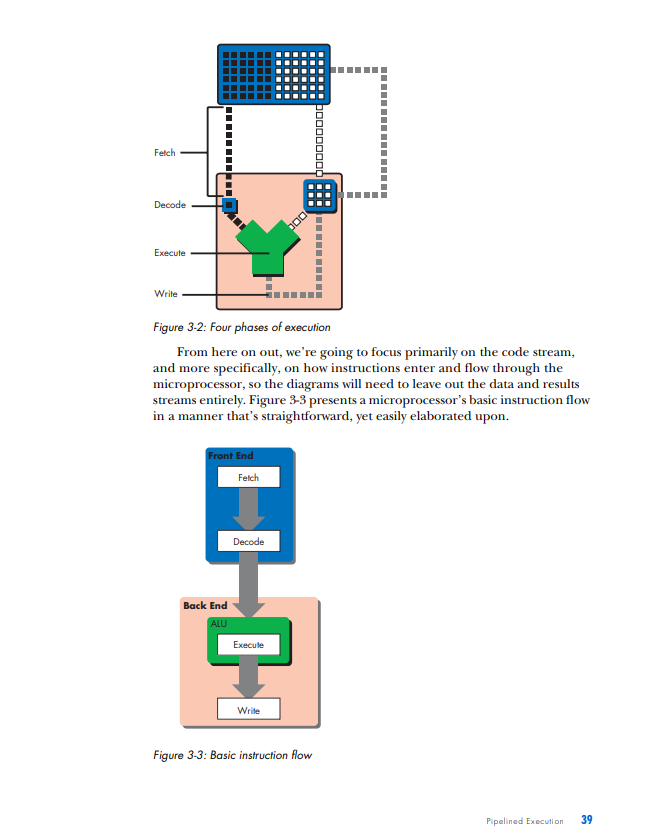
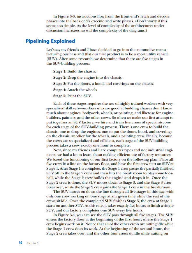
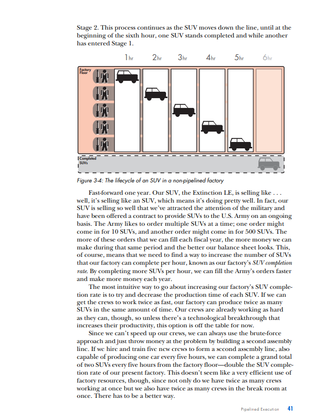
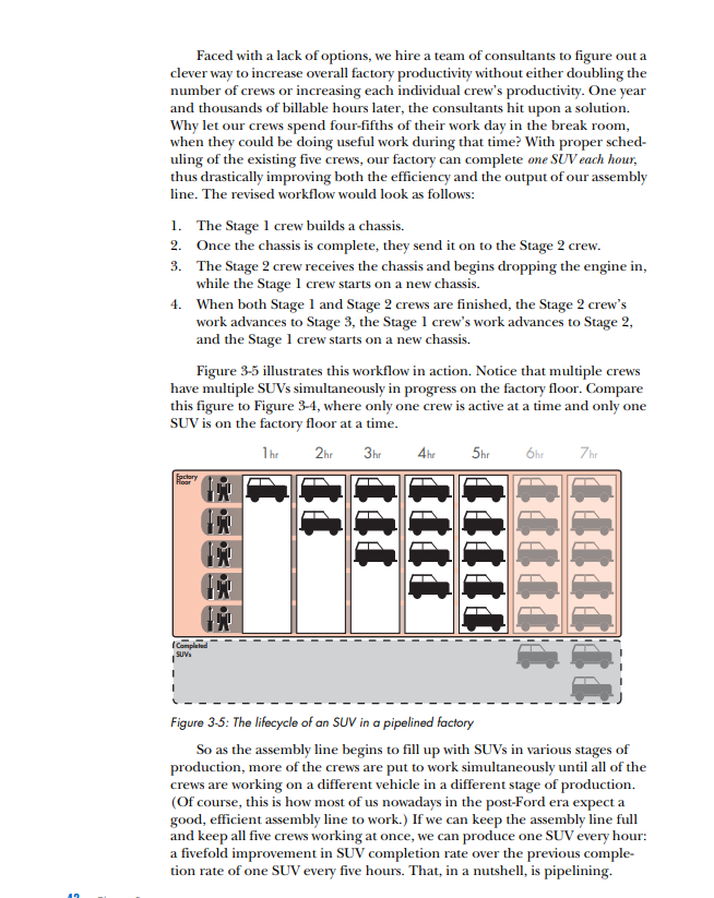
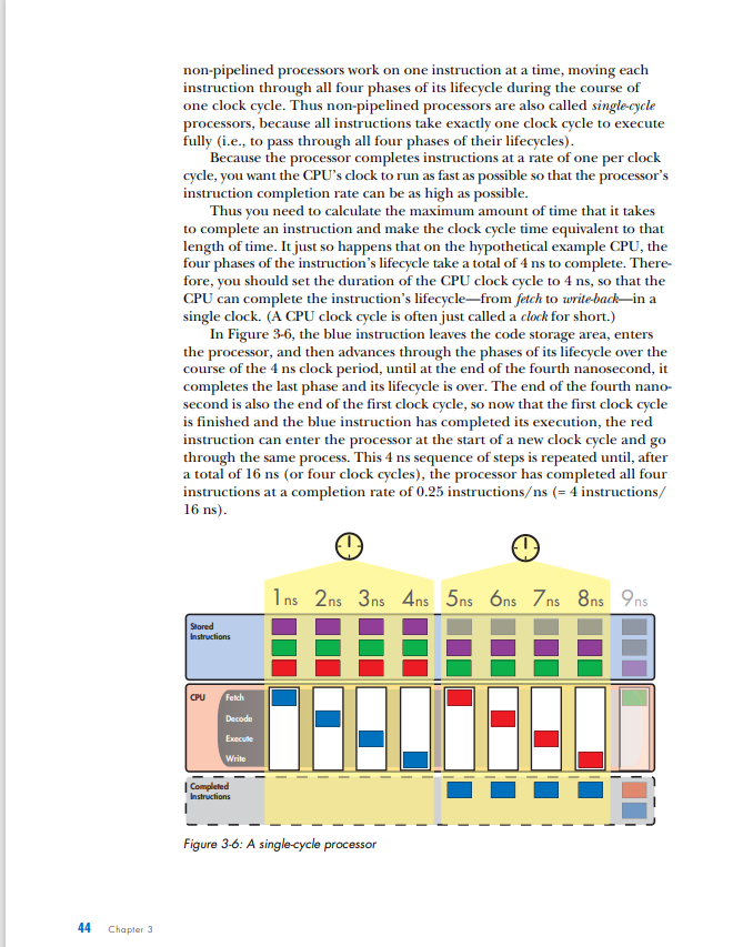
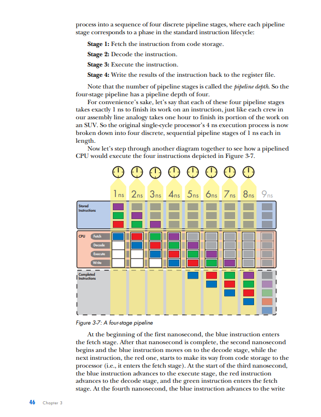
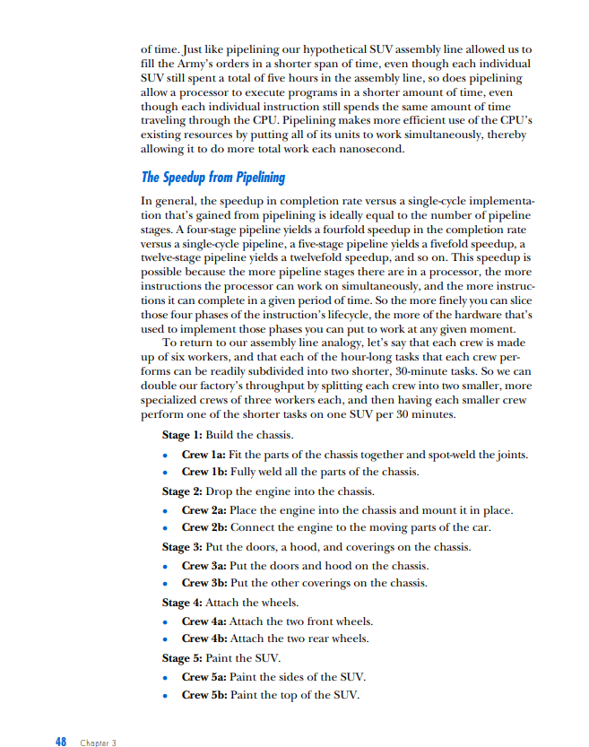
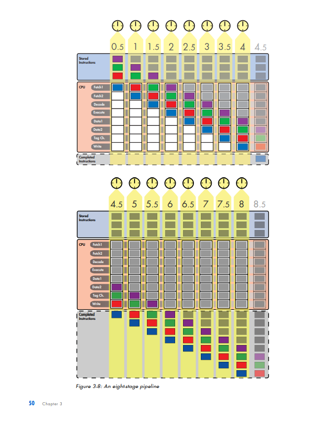
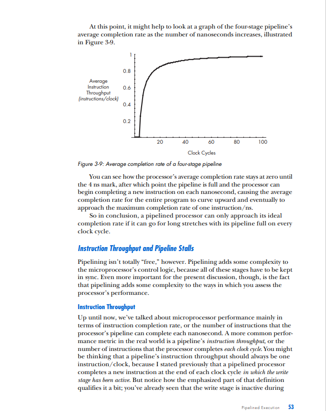
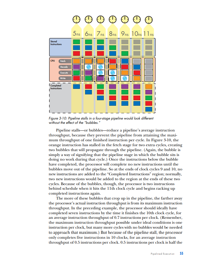
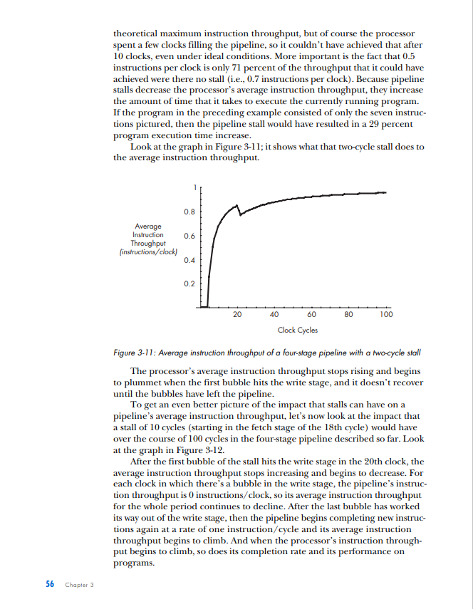
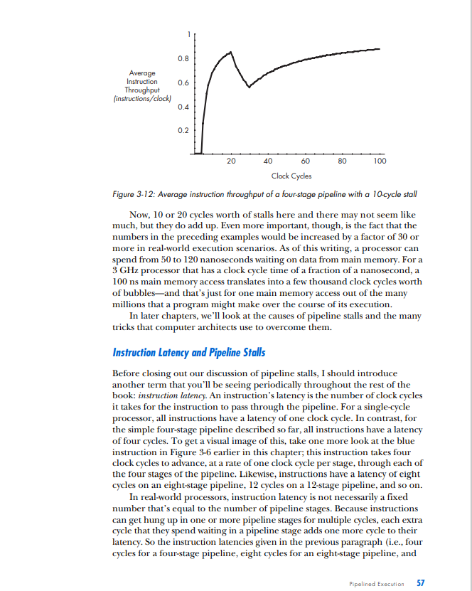
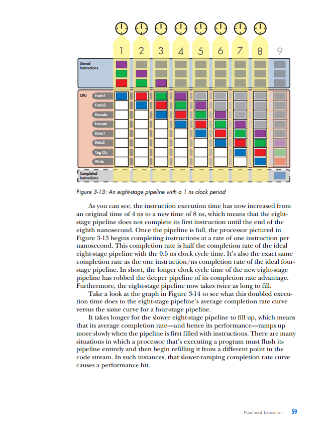
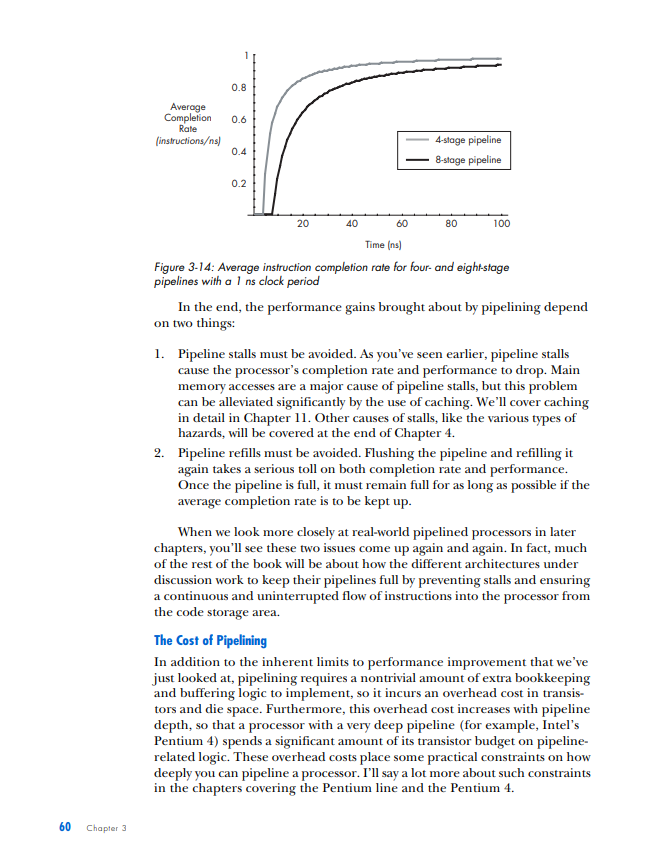
PIPELINED EXECUTION All of the processor architectures that you've looked at so far are relatively simple, and they reflect the earliest stages of computer evolution. This chapter will bring you closer to the modern computing era by introducing one of the key innovations that underlies the rapid performance increases that have characterized the past few decades of microprocessor development: pipelined execution. Pipelined execution is a technique that enables microprocessor designers to increase the speed at which a processor operates, thereby decreasing the amount of time that the processor takes to execute a program. This chapter will first introduce the concept of pipelining by means of a factory analogy, and it will then apply the analogy to microprocessors. You'll then learn how to evaluate the benefits of pipelining, before I conclude with a discussion of the technique's limitations and costs. NOTE This chapter's discussion of pipelined execution focuses solely on the execution of arith metic instructions. Memory instructions and branch instructions are pipelined using the same fundamental principles as arithmetic instructions, and later chapters will cover the peculiarities of the actual execution process of each of these two types of instruction. In the previous chapter, you learned that a computer repeats three basic steps over and over again in order to execute a program: 1. Fetch the next instruction from the address stored in the program counter and load that instruction into the instruction register. Increment the program counter. 2. Decode the instruction in the instruction register. 3. Execute the instruction in the instruction register. You should also recall that step 3, the execute step, itself can consist of multiple sub-steps, depending on the type of instruction being executed (arithmetic, memory access, or branch). In the case of the arithmetic instruction add A,B,C, the example we used last time, the three sub-steps are as follows: 1. Read the contents of registers A and B. 2. Add the contents of A and B. 3. Write the result back to register C. Thus the expanded list of actions required to execute an arithmetic instruction is as follows (substitute any other arithmetic instruction for add in the following list to see how it's executed): 1. Fetch the next instruction from the address stored in the program counter and load that instruction into the instruction register. Increment the program counter. 2. Decode the instruction in the instruction register. 3. Execute the instruction in the instruction register. Because the instruction is not a branch instruction but an arithmetic instruction, send it to the arithmetic logic unit (ALU). a. Read the contents of registers A and B. b. Add the contents of A and B. c. Write the result back to register C. At this point, I need to make a modification to the preceding list. For reasons we'll discuss in detail when we talk about the instruction window in Chapter 5, most modern microprocessors treat sub-steps 3a and 3b as a group, while they treat step 3c, the register write, separately. To reflect this conceptual and architectural division, this list should be modified to look as follows: 1. Fetch the next instruction from the address stored in the program counter, and load that instruction into the instruction register. Increment the program counter. 2. Decode the instruction in the instruction register. 3. Execute the instruction in the instruction register. Because the instruction is not a branch instruction but an arithmetic instruction, send it to the ALU. a. Read the contents of registers A and B. b. Add the contents of A and B. 4. Write the result back to register C. In a modern processor, these four steps are repeated over and over again until the program is finished executing. These are, in fact, the four stages in a classic RISC 1 pipeline. (I'll define the term pipeline shortly; for now, just think of a pipeline as a series of stages that each instruction in the code stream must pass through when the code stream is being executed.) Here are the four stages in their abbreviated form, the form in which you'll most often see them: 1. Fetch 2. Decode 3. Execute 4. Write (or "write-back") Each of these stages could be said to represent one phase in the lifecycle of an instruction. An instruction starts out in the fetch phase, moves to the decode phase, then to the execute phase, and finally to the write phase. As I mentioned in "The Clock" on page 29, each phase takes a fixed, but by no means equal, amount of time. In most of the example processors with which you'll be working in this chapter, all four phases take an equal amount of time; this is not usually the case in real-world processors. In any case, if the DLW-1 takes exactly 1 nanosecond (ns) to complete each phase, then the DLW-1 can finish one instruction every 4ns. 1 The term RISC is an acronym for Reduced Instruction Set Computing. I'll cover this term in more detail in Chapter 5. ic Instruction Flow One useful division that computer architects often employ when talking about CPUs is that of front end versus back end. As you already know, when instructions are fetched from main memory, they must be decoded for execution. This fetching and decoding takes place in the processor's front end. You can see in Figure 3-1 that the front end roughly corresponds to the control and I/O units in the previous chapter's diagram of the DLW-l's programming model. The ALU and registers constitute the back end of the DLW-1. Instructions make their way from the front end down through the back end, where the work of number crunching gets done. Figure 3-1: Front end versus back end We can now modify Figure 1-4 to show all four phases of execution (see Figure 3-2). Figure 3-2: Four phases of execufion From here on out, we're going to focus primarily on the code stream, and more specifically, on how instructions enter and flow through the microprocessor, so the diagrams will need to leave out the data and results streams entirely. Figure 3-3 presents a microprocessor's basic instruction flow in a manner that's straightforward, yet easily elaborated upon. Figure 3-3: Basic instruction flow In Figure 3-3, instructions flow from the front end's fetch and decode phases into the back end's execute and write phases. (Don't worry if this seems too simple. As the level of complexity of the architectures under discussion increases, so will the complexity of the diagrams.) Explained Let's say my friends and I have decided to go into the automotive manufacturing business and that our first product is to be a sport utility vehicle (SUV). After some research, we determine that there are five stages in the SUV-building process: Stage 1: Build the chassis. Stage 2: Drop the engine into the chassis. Stage 3: Put the doors, a hood, and coverings on the chassis. Stage 4: Attach the wheels. Stage 5: Paint the SUV. Each of these stages requires the use of highly trained workers with very specialized skill sets-workers who are good at building chasses don't know much about engines, bodywork, wheels, or painting, and likewise for engine builders, painters, and the other crews. So when we make our first attempt to put together an SUV factory, we hire and train five crews of specialists, one for each stage of the SUV-building process. There's one crew to build the chassis, one to drop the engines, one to put the doors, hood, and coverings on the chassis, another for the wheels, and a painting crew. Finally, because the crews are so specialized and efficient, each stage of the SUV-building process takes a crew exactly one hour to complete. Now, since my friends and I are computer types and not industrial engineers, we had a lot to learn about making efficient use of factory resources. We based the functioning of our first factory on the following plan: Place all five crews in a line on the factory floor, and have the first crew start an SUV at Stage 1 . After Stage 1 is complete, the Stage 1 crew passes the partially finished SUV off to the Stage 2 crew and then hits the break room to play some foosball, while the Stage 2 crew builds the engine and drops it in. Once the Stage 2 crew is done, the SUV moves down to Stage 3 , and the Stage 3 crew takes over, while the Stage 2 crew joins the Stage 1 crew in the break room. The SUV moves on down the line through all five stages in this way, with only one crew working on one stage at any given time while the rest of the crews sit idle. Once the completed SUV finishes Stage 5, the crew at Stage 1 starts on another SUV. At this rate, it takes exactly five hours to finish a single SUV, and our factory completes one SUV every five hours. In Figure 3-4, you can see the SUV pass through all five stages. The SUV enters the factory floor at the beginning of the first hour, where the Stage 1 crew begins work on it. Notice that all of the other crews are sitting idle while the Stage 1 crew does its work. At the beginning of the second hour, the Stage 2 crew takes over, and the other four crews sit idle while waiting on Stage 2. This process continues as the SUV moves down the line, until at the beginning of the sixth hour, one SUV stands completed and while another has entered Stage 1. Figure 3-4: The lifecycle of an SUV in a non-pipelined factory Fast-forward one year. Our SUV, the Extinction LE, is selling like... well, it's selling like an SUV, which means it's doing pretty well. In fact, our SUV is selling so well that we've attracted the attention of the military and have been offered a contract to provide SUVs to the U.S. Army on an ongoing basis. The Army likes to order multiple SUVs at a time; one order might come in for 10 SUVs, and another order might come in for 500 SUVs. The more of these orders that we can fill each fiscal year, the more money we can make during that same period and the better our balance sheet looks. This, of course, means that we need to find a way to increase the number of SUVs that our factory can complete per hour, known as our factory's SUV completion rate. By completing more SUVs per hour, we can fill the Army's orders faster and make more money each year. The most intuitive way to go about increasing our factory's SUV completion rate is to try and decrease the production time of each SUV. If we can get the crews to work twice as fast, our factory can produce twice as many SUVs in the same amount of time. Our crews are already working as hard as they can, though, so unless there's a technological breakthrough that increases their productivity, this option is off the table for now. Since we can't speed up our crews, we can always use the brute-force approach and just throw money at the problem by building a second assembly linc. If wc hirc and train fivc ncw crews to form a sccond asscmbly linc, also capable of producing one car every five hours, we can complete a grand total of two SUVs every five hours from the factory floor-double the SUV completion rate of our present factory. This doesn't seem like a very efficient use of factory resources, though, since not only do we have twice as many crews working at once but we also have twice as many crews in the break room at once. There has to be a better way. Faced with a lack of options, we hire a team of consultants to figure out a clever way to increase overall factory productivity without either doubling the number of crews or increasing each individual crew's productivity. One year and thousands of billable hours later, the consultants hit upon a solution. Why let our crews spend four-fifths of their work day in the break room, when they could be doing useful work during that time? With proper scheduling of the existing five crews, our factory can complete one SUV each hour, thus drastically improving both the efficiency and the output of our assembly line. The revised workflow would look as follows: 1. The Stage 1 crew builds a chassis. 2. Once the chassis is complete, they send it on to the Stage 2 crew. 3. The Stage 2 crew receives the chassis and begins dropping the engine in, while the Stage 1 crew starts on a new chassis. 4. When both Stage 1 and Stage 2 crews are finished, the Stage 2 crew's work advances to Stage 3, the Stage 1 crew's work advances to Stage 2, and the Stage 1 crew starts on a new chassis. Figure 35 illustrates this workflow in action. Notice that multiple crews have multiple SUVs simultaneously in progress on the factory floor. Compare this figure to Figure 3-4, where only one crew is active at a time and only one SUV is on the factory floor at a time. Figure 3-5: The lifecycle of an SUV in a pipelined factory So as the assembly line begins to fill up with SUVs in various stages of production, more of the crews are put to work simultaneously until all of the crews are working on a different vehicle in a different stage of production. (Of course, this is how most of us nowadays in the post-Ford era expect a good, efficient assembly line to work.) If we can keep the assembly line full and keep all five crews working at once, we can produce one SUV every hour: a fivefold improvement in SUV completion rate over the previous completion rate of one SUV every five hours. That, in a nutshell, is pipelining. While the total amount of time that each individual SUV spends in production has not changed from the original five hours, the rate at which the factory as a whole completes SUVs has increased drastically. Furthermore, the rate at which the factory can fulfill the Army's orders for batches of SUVs has increased drastically, as well. Pipelining works its magic by making optimal use of already existing resources. We don't need to speed up each individual stage of the production process, nor do we need to drastically increase the amount of resources that we throw at the problem; all that's necessary is that we get more work out of resources that are already there. WHY THE SUV FACTORY? The preceding discussion uses a factory analogy to explain pipelining. Other books use simpler analogies, like doing laundry, for instance, to explain this technique, but there are a few reasons why I chose a more elaborate and lengthy analogy to illustrate what is a relatively simple concept. First, I use factory analogies throughout this book, because assembly line-based factories are easy for readers to visualize and there's plenty of room for filling out the mental image in interesting ways in order to make a variety of related points. Second, and perhaps even more importantly, the many scheduling-, queving- and resource management-related problems that factory designers face have direct analogies in computer architecture. In many cases, the problems and solutions are exactly the same, simply translated into a different domain. (Similar queuingrelated problem/solution pairs also crop up in the service industry, which is why analogies involving supermarkets and fast food restaurants are also favorites of mine.) Bringing our discussion back to microprocessors, it should be easy to see how this concept applies to the four phases of an instruction's lifecycle. Just as the owners of the factory in our analogy wanted to increase the number of SUVs that the factory could finish in a given period of time, microprocessor designers are always looking for ways to increase the number of instructions that a CPU can complete in a given period of time. When you recall that a program is an ordered sequence of instructions, it becomes clear that increasing the number of instructions executed per unit time is one way to decrease the total amount of time that it takes to execute a program. (The other way to decrease a program's execution time is to decrease the number of instructions in the program, but this chapter won't address that approach until later.) In terms of our analogy, a program is like an order of SUVs from the military; just like increasing our factory's output of SUVs per hour enabled us to fill orders faster, increasing a processor's instruction completion rate (the number of instructions completed per unit time) enables it to run programs faster. A Non-Pipelined Processor The previous chapter briefly described how the simple processors described so far (e.g., the DLW=1) use the clock to time its internal operations. These non-pipelined processors work on one instruction at a time, moving each instruction through all four phases of its lifecycle during the course of one clock cycle. Thus non-pipelined processors are also called singlecycle processors, because all instructions take exactly one clock cycle to execute fully (i.e., to pass through all four phases of their lifecycles). Because the processor completes instructions at a rate of one per clock cycle, you want the CPU's clock to run as fast as possible so that the processor's instruction completion rate can be as high as possible. Thus you need to calculate the maximum amount of time that it takes to complete an instruction and make the clock cycle time equivalent to that length of time. It just so happens that on the hypothetical example CPU, the four phases of the instruction's lifecycle take a total of 4 ns to complete. Therefore, you should set the duration of the CPU clock cycle to 4ns, so that the CPU can complete the instruction's lifecycle-from fetch to write-back-in a single clock. (A CPU clock cycle is often just called a clock for short.) In Figure 3-6, the blue instruction leaves the code storage area, enters the processor, and then advances through the phases of its lifecycle over the course of the 4ns clock period, until at the end of the fourth nanosecond, it completes the last phase and its lifecycle is over. The end of the fourth nanosecond is also the end of the first clock cycle, so now that the first clock cycle is finished and the blue instruction has completed its execution, the red instruction can enter the processor at the start of a new clock cycle and go through the same process. This 4ns sequence of steps is repeated until, after a total of 16ns (or four clock cycles), the processor has completed all four instructions at a completion rate of 0.25 instructionss (= 4 instructions/ 16ns ). Single-cycle processors like the one in Figure 3-6 are simple to design, but they waste a lot of hardware resources. All of that white space in the diagram represents processor hardware that's sitting idle while it waits for the instruction that's currently in the processor to finish executing. By pipelining the processor in this figure, you can put more of that hardware to work every nanosecond, thereby increasing the processor's efficiency and its performance on executing programs. Before moving on, I should clarify a few concepts illustrated in Figure 3-6. At the bottom is a region labeled "Completed Instructions." Completed instructions don't actually go anywhere when they're finished executing; once they've done their job of telling the processor how to modify the data stream, they're simply deleted from the processor. So the "Completed Instructions" box does not represent a real part of the computer, which is why I've placed a dotted line around it. This area is just a place for you to keep track of how many instructions the processor has completed in a certain amount of time, or the processor's instruction completion rate (or completion rate, for short), so that when you compare different types of processors, you'll have a place where you can quickly see which processor performs better. The more instructions a processor completes in a set amount of time, the better it performs on programs, which are an ordered sequence of instructions. Think of the "Completed Instructions" box as a sort of scoreboard for tracking each processor's completion rate, and check the box in each of the subsequent figures to see how long it takes for the processor to populate this box. Following on the preceding point, you may be curious as to why the blue instruction that has completed in the fourth nanosecond does not appear in the "Completed Instructions" box until the fifth nanosecond. The reason is straightforward and stems from the nature of the diagram. Because an instruction spends one complete nanosecond, from start to finish, in each stage of execution, the blue instruction enters the write phase at the beginning of the fourth nanosecond and exits the write phase at the end of the fourth nanosecond. This means that the fifth nanosecond is the first full nanosecond in which the blue instruction stands completed. Thus at the beginning of the fifth nanosecond (which coincides with the end of the fourth nanosecond), the processor has completed one instruction. A Pipelined Processor Pipelining a processor means breaking down its instruction execution process-what I've been calling the instruction's lifecycle-into a series of discrete pipeline stages that can be completed in sequence by specialized hardware. Recall the way that we broke down the SUV assembly process into five discrete steps - with one dedicated crew assigned to complete each stepand you'll get the idea. Because an instruction's lifecycle consists of four fairly distinct phases, you can start by breaking down the single-cycle processor's instruction execution Pipelined Exacution 45 process into a sequence of four discrete pipeline stages, where each pipeline stage corresponds to a phase in the standard instruction lifecycle: Stage 1: Fetch the instruction from code storage. Stage 2: Decode the instruction. Stage 3: Execute the instruction. Stage 4: Write the results of the instruction back to the register file. Note that the number of pipeline stages is called the pipeline depth. So the four-stage pipeline has a pipeline depth of four. For convenience's sake, let's say that each of these four pipeline stages takes exactly 1 ns to finish its work on an instruction, just like each crew in our assembly line analogy takes one hour to finish its portion of the work on an SUV. So the original single-cycle processor's 4ns execution process is now broken down into four discrete, sequential pipeline stages of 1 ns each in length. Now let's step through another diagram together to see how a pipelined CPU would execute the four instructions depicted in Figure 3-7. Figure 3-7: A four-stage pipeline At the beginning of the first nanosecond, the blue instruction enters the fetch stage. After that nanosecond is complete, the second nanosecond begins and the blue instruction moves on to the decode stage, while the next instruction, the red one, starts to make its way from code storage to the processor (i.e., it enters the fetch stage). At the start of the third nanosecond, the blue instruction advances to the execute stage, the red instruction advances to the decode stage, and the green instruction enters the fetch stage. At the fourth nanosecond, the blue instruction advances to the write stage, the red instruction advances to the execute stage, the green instruction advances to the decode stage, and the purple instruction advances to the fetch stage. After the fourth nanosecond has fully elapsed and the fifth nanosecond starts, the blue instruction has passed from the pipeline and is now finished executing. Thus we can say that at the end of 4ns (= four clock cycles), the pipelined processor depicted in Figure 3-7 has completed one instruction. At start of the fifth nanosecond, the pipeline is now full and the processor can begin completing instructions at a rate of one instruction per nanosecond. This one instructions completion rate is a fourfold improvement over the single-cycle processor's completion rate of 0.25 instructionss (or four instructions every 16ns ). Shrinking the Clock You can see from Figure 3-7 that the role of the CPU clock changes slightly in a pipelined processor, compared to the single-cycle processor shown in Figure 3-6. Because all of the pipeline stages must now work together simultaneously and be ready at the start of each new nanosecond to hand over the results of their work to the next pipeline stage, the clock is needed to coordinate the activity of the whole pipeline. The way this is done is simple: Shrink the clock cycle time to match the time it takes each stage to complete its work so that at the start of each clock cycle, each pipeline stage hands off the instruction it was working on to the next stage in the pipeline. Because each pipeline stage in the example processor takes 1 ns to complete its work, you can set the clock cycle to be 1 ns in duration. This new method of clocking the processor means that a new instruction will not necessarily be completed at the close of each clock cycle, as was the case with the single-cycle processor. Instead, a new instruction will be completed at the close of only those clock cycles in which the write stage has been working on an instruction. Any clock cycle with an empty write stage will add no new instructions to the "Completed Instructions" box, and any clock cycle with an active write stage will add one new instruction to the box. Of course, this means that when the pipeline first starts to work on a program, there will be a few clock cycles-three to be exact-during which no instructions are completed. But once the fourth clock cycle starts, the first instruction enters the write stage and the pipeline can then begin completing new instructions on each clock cycle, which, because each clock cycle is 1ns, translates into a completion rate of one instruction per nanosecond. Shrinking Program Execution Time Note that the total execution time for each individual instruction is not changed by pipelining. It still takes an instruction 4ns to make it all the way through the processor; that 4ns can be split up into four clock cycles of 1ns each, or it can cover one longer clock cycle, but it's still the same 4 ns. Thus pipelining doesn't speed up instruction execution time, but it does speed up program execution time (the number of nanoseconds that it takes to execute an entire program) by increasing the number of instructions finished per unit Pipelined Execution 47 of time. Just like pipelining our hypothetical SUV assembly line allowed us to fill the Army's orders in a shorter span of time, even though each individual SUV still spent a total of five hours in the assembly line, so does pipelining allow a processor to execute programs in a shorter amount of time, even though each individual instruction still spends the same amount of time traveling through the CPU. Pipelining makes more efficient use of the CPU's existing resources by putting all of its units to work simultaneously, thereby allowing it to do more total work each nanosecond. The Speedup from Pipelining In general, the speedup in completion rate versus a single-cycle implementation that's gained from pipelining is ideally equal to the number of pipeline stages. A four-stage pipeline yields a fourfold speedup in the completion rate versus a single-cycle pipeline, a five-stage pipeline yields a fivefold speedup, a twelve-stage pipeline yields a twelvefold speedup, and so on. This speedup is possible because the more pipeline stages there are in a processor, the more instructions the processor can work on simultaneously, and the more instructions it can complete in a given period of time. So the more finely you can slice those four phases of the instruction's lifecycle, the more of the hardware that's used to implement those phases you can put to work at any given moment. To return to our assembly line analogy, let's say that each crew is made up of six workers, and that each of the hour-long tasks that each crew performs can be readily subdivided into two shorter, 30-minute tasks. So we can double our factory's throughput by splitting each crew into two smaller, more specialized crews of three workers each, and then having each smaller crew perform one of the shorter tasks on one SUV per 30 minutes. Stage 1: Build the chassis. - Crew 1a: Fit the parts of the chassis together and spot-weld the joints. - Crew 1b: Fully weld all the parts of the chassis. Stage 2: Drop the engine into the chassis. - Crew 2a: Place the engine into the chassis and mount it in place. - Crew 2b: Connect the engine to the moving parts of the car. Stage 3: Put the doors, a hood, and coverings on the chassis. - Crew 3a: Put the doors and hood on the chassis. - Crew 3b: Put the other coverings on the chassis. Stage 4: Attach the wheels. - Crew 4a: Attach the two front wheels. - Crew 4b: Attach the two rear wheels. Stage 5: Paint the SUV. - Crew 5a: Paint the sides of the SUV. - Crew 5b: Paint the top of the SUV. After the modifications described here, the 10 smaller crews in our factory now have a collective total of 10SUVs in progress during the course of any given 30-minute period. Furthermore, our factory can now complete a new SUV every 30 minutes, a tenfold improvement over our first factory's completion rate of one SUV every five hours. So by pipelining our assembly line even more deeply, we've put even more of its workers to work concurrently, thereby increasing the number of SUVs that can be worked on simultaneously and increasing the number of SUVs that can be completed within a given period of time. Deepening the pipeline of the four-stage processor works on similar principles and has a similar effect on completion rates. Just as the five stages in our SUV assembly line could be broken down further into a longer sequence of more specialized stages, the execution process that each instruction goes through can be broken down into a series of much more than just four discrete stages. By breaking the processor's four-stage pipeline down into a longer series of shorter, more specialized stages, even more of the processor's specialized hardware can work simultaneously on more instructions and thereby increase the number of instructions that the pipeline completes each nanosecond. We first moved from a single-cycle processor to a pipelined processor by taking the 4ns time period that the instruction spent traveling through the processor and slicing it into four discrete pipeline stages of 1ns each in length. These four discrete pipeline stages corresponded to the four phases of an instruction's lifecycle. A processor's pipeline stages aren't always going to correspond exactly to the four phases of a processor's lifecycle, though. Some processors have a five-stage pipeline, some have a six-stage pipeline, and many have pipelines deeper than 10 or 20 stages. In such cases, the CPU designer must slice up the instruction's lifecycle into the desired number of stages in such a way that all the stages are equal in length. Now let's take that 4ns execution process and slice it into eight discrete stages. Because all eight pipeline stages must be of exactly the same duration for pipelining to work, the eight pipeline stages must each be 4ns8=0.5ns in length. Since we're presently working with an idealized example, let's pretend that splitting up the processor's four-phase lifecycle into eight equally long ( 0.5ns) pipeline stages is a trivial matter, and that the results look like what you see in Figure 3-8. (In reality, this task is not trivial and involves a number of trade-offs. As a concession to that reality, I've chosen to use the eight stages of a real-world pipeline-the MIPS pipeline-in Figure 3-8, instead of just splitting each of the four traditional stages in two.) Because pipelining requires that each pipeline stage take exactly one clock cycle to complete, the clock cycle can now be shortened to 0.5ns in order to fit the lengths of the eight pipeline stages. At the bottom of Figure 3-8, you can see the impact that this increased number of pipeline stages has on the number of instructions completed per unit time. Figure 3.8: An eight-stage pipoline 50 Chapter 3 The single-cycle processor can complete one instruction every 4ns, for a completion rate of 0.25 instructionss, and the four-stage pipelined processor can complete one instruction every nanosecond for a completion rate of one instructionss. The eight-stage processor depicted in Figure 3-8 improves on both of these by completing one instruction every 0.5ns, for a completion rate of two instructionss. Note that because each instruction still takes 4ns to execute, the first 4ns of the eight-stage processor are still dedicated to filling up the pipeline. But once the pipeline is full, the processor can begin completing instructions twice as fast as the four-stage processor and eight times as fast as the single-stage processor. This eightfold increase in completion rate versus a single-cycle design means that the eight-stage processor can execute programs much faster than either a single-cycle or a four-stage processor. But does the eightfold increase in completion rate translate into an eightfold increase in processor performance? Not exactly. Program Execution Time and Completion Rate If the program that the single-cycle processor in Figure 3-6 is running consisted of only the four instructions depicted, that program would have a program execution time of 16ns, or 4 instructions 0.25 instructions s. If the program consisted of, say, seven instructions, it would have a program execution time of 7 instructions 0.25 instructions s=28ns. In general, a program's execution time is equal to the total number of instructions in the program divided by the processor's instruction completion rate (number of instructions completed per nanosecond), as in the following equation: program execution time = number of instructions in program / instruction completion rate Most of the time, when I talk about processor performance in this book, I'm talking about program execution time. One processor performs better than another if it executes all of a program's instructions in a shorter amount of time, so reducing program execution time is the key to increasing processor performance. From the preceding equation, it should be clear that program execution time can be reduced in one of two ways: by a reduction in the number of instructions per program or by an increase in the processor's completion rate. For now, let's assume that the number of instructions in a program is fixed and that there's nothing that can be done about this term of the equation. As such, our focus in this chapter will be on increasing instruction completion rates. In the case of a non-pipelined, singlecycle processor, the instruction completion rate ( x instructions per 1ns ) is simply the inverse of the instruc execuL me ( y us per 1 insu uction), where x and y have different numerical values. Because the relationship between completion rate and instruction execution time is simple and direct in a single-cycle processor, an n fold improvement in one is an nfold improvement in the other. So improving the performance of a single-cycle processor is really about reducing instruction execution times. With pipelined processors, the relationship between instruction execution time and completion rate is more complex. As discussed previously, pipelined processors allow you to increase the processor's completion rate without altering the instruction execution time. Of course, a reduction in instruction execution time still translates into a completion rate improvement, but the reverse is not necessarily true. In fact, as you'll learn later on, pipelining's improvements to completion rate often come at the price of increased instruction execution times. This means that for pipelining to improve performance, the processor's completion rate must be as high as possible over the course of a program's execution. The Relationship Between Completion Rate and Program Execution Time If you look at the "Completed Instructions" box of the four-stage processor back in Figure 3-7, you'll see that a total of five instructions have been completed at the start of the ninth nanosecond. In contrast, the non-pipelined processor illustrated in Figure 3-6 sports two completed instructions at the start of the ninth nanosecond. Five completed instructions in the span of 8ns is obviously not a fourfold improvement over two completed instructions in the same time period, so what gives? Remember that it took the pipelined processor 4ns initially to fill up with instructions; the pipelined processor did not complete its first instruction until the end of the fourth nanosecond. Therefore, it completed fewer instructions over the first 8ns of that program's execution than it would have had the pipeline been full for the entire 8ns. When the processor is executing programs that consist of thousands of instructions, then as the number of nanoseconds stretches into the thousands, the impact on program execution time of those four initial nanoseconds, during which only one instruction was completed, begins to vanish and the pipelined processor's advantage begins to approach the fourfold mark. For example, after 1,000ns, the non-pipelined processor will have completed 250 instructions ( 1000ns0.25 instructions s=250 instructions), while the pipelined processor will have completed 996 instructions [(1000ns4ns)1 instructionss] a 3.984-fold improvement. What I've just described using this concrete example is the difference between a pipeline's maximum theoretical completion rate and its real-world average completion rate. In the previous example, the four-stage processor's maximum theoretical completion rate, i.e., its completion rate on cycles when its entire pipeline is full, is one instructions. However, the processor's average compltion rat during its first 8ns is 5 instructions/ 8 ns 0.625 instructionss. The processor's average completion rate improves as it passes more clock cycles with its pipeline full, until at 1,000ns, its average completion rate is 996 instructions/ 1000ns=0.996 instructionss. At this point, it might help to look at a graph of the four-stage pipeline's average completion rate as the number of nanoseconds increases, illustrated in Figure 3-9. Figure 3-9: Average completion rate of a four-stage pipeline You can see how the processor's average completion rate stays at zero until the 4ns mark, after which point the pipeline is full and the processor can begin completing a new instruction on each nanosecond, causing the average completion rate for the entire program to curve upward and eventually to approach the maximum completion rate of one instructions. So in conclusion, a pipelined processor can only approach its ideal completion rate if it can go for long stretches with its pipeline full on every clock cycle. Instruction Throughput and Pipeline Stalls Pipelining isn't totally "free," however. Pipelining adds some complexity to the microprocessor's control logic, because all of these stages have to be kept in sync. Even more important for the present discussion, though, is the fact that pipelining adds some complexity to the ways in which you assess the processor's performance. Instruction Throughput Up until now, we've talked about microprocessor performance mainly in terms of instruction completion rate, or the number of instructions that the processor's pipeline can complete each nanosecond. A more common performance metric in the real world is a pipeline's instruction throughput, or the number of instructions that the processor completes each clock cycle. You might be thinking that a pipeline's instruction throughput should always be one instruction/clock, because I stated previously that a pipelined processor completes a new instruction at the end of each clock cycle in which the write stage has been active. But notice how the emphasized part of that definition qualifies it a bit; you've already seen that the write stage is inactive during clock cycles in which the pipeline is being filled, so on those clock cycles, the processor's instruction throughput is 0 instructions/clock. In contrast, when the instruction's pipeline is full and the write stage is active, the pipelined processor has an instruction throughput of 1 instruction/clock. So just like there was a difference between a processor's maximum theoretical completion rate and its average completion rate, there's also a difference between a processor's maximum theoretical instruction throughput and its average instruction throughput: Instruction throughput The number of instructions that the processor finishes executing on each clock cycle. You'll also see instruction throughput referred to as instructions per clock (IPC). Maximum theoretical instruction throughput The theoretical maximum number of instructions that the processor can finish executing on each clock cycle. For the simple kinds of pipelined and non-pipelined processors described so far, this number is always one instruction per cycle (one instruction/clock or one IPC). Average instruction throughput The average number of instructions per clock (IPC) that the processor has actually completed over a certain number of cycles. A processor's instruction throughput is closely tied to its instruction completion rate-the more instructions that the processor completes each clock cycle (instructions/clock), the more instructions it also completes over a given period of time (instructionss). We'll talk more about the relationship between these two metrics in a moment, but for now just remember that a higher instruction throughput translates into a higher instruction completion rate, and hence better performance. Pipeline Stalls In the real world, a processor's pipeline can be found in more conditions than just the two described so far: a full pipeline or a pipeline that's being filled. Sometimes, instructions get hung up in one pipeline stage for multiple cycles. There are a number of reasons why this might happen-we'll discuss many of them throughout this book-but when it happens, the pipeline is said to stall. When the pipeline stalls, or gets hung in a certain stage, all of the instructions in the stages below the one where the stall happened continue advancing normally, while the stalled instruction just sits in its stage, and all the instructions behind it back up. In Figure 3-10, the orange instruction is stalled for two extra cycles in the fetch stage. Because the instruction is stalled, a new gap opens ahead of it in the pipeline for each cycle that it stalls. Once the instruction starts advancing through the pipeline again, the gaps in the pipeline that were created by the stall-gaps that are commonly called "pipeline bubbles"-travel down the pipeline ahead of the formerly stalled instruction until they eventually leave the pipeline. without the effect of the "bubbles." Pipeline stalls-or bubbles-reduce a pipeline's average instruction throughput, because they prevent the pipeline from attaining the maximum throughput of one finished instruction per cycle. In Figure 3-10, the orange instruction has stalled in the fetch stage for two extra cycles, creating two bubbles that will propagate through the pipeline. (Again, the bubble is simply a way of signifying that the pipeline stage in which the bubble sits is doing no work during that cycle.) Once the instructions below the bubble have completed, the processor will complete no new instructions until the bubbles move out of the pipeline. So at the ends of clock cycles 9 and 10 , no new instructions are added to the "Completed Instructions" region; normally, two new instructions would be added to the region at the ends of these two cycles. Because of the bubbles, though, the processor is two instructions behind schedule when it hits the 11 th clock cycle and begins racking up completed instructions again. The more of these bubbles that crop up in the pipeline, the farther away the processor's actual instruction throughput is from its maximum instruction throughput. In the preceding example, the processor should ideally have completed seven instructions by the time it finishes the 10 th clock cycle, for an average instruction throughput of 0.7 instructions per clock. (Remember, the maximum instruction throughput possible under ideal conditions is one instruction per clock, but many more cycles with no bubbles would be needed t approach that maximum.) But beecause of the pipeeline stall, th processor only completes five instructions in 10 clocks, for an average instruction throughput of 0.5 instructions per clock. 0.5 instructions per clock is half the theoretical maximum instruction throughput, but of course the processor spent a few clocks filling the pipeline, so it couldn't have achieved that after 10 clocks, even under ideal conditions. More important is the fact that 0.5 instructions per clock is only 71 percent of the throughput that it could have achieved were there no stall (i.e., 0.7 instructions per clock). Because pipeline stalls decrease the processor's average instruction throughput, they increase the amount of time that it takes to execute the currently running program. If the program in the preceding example consisted of only the seven instructions pictured, then the pipeline stall would have resulted in a 29 percent program execution time increase. Look at the graph in Figure 3-11; it shows what that two-cycle stall does to the average instruction throughput. Figure 3-11: Average instruction throughput of a four-stage pipeline with a two-cycle stall The processor's average instruction throughput stops rising and begins to plummet when the first bubble hits the write stage, and it doesn't recover until the bubbles have left the pipeline. To get an even better picture of the impact that stalls can have on a pipeline's average instruction throughput, let's now look at the impact that a stall of 10 cycles (starting in the fetch stage of the 18th cycle) would have over the course of 100 cycles in the four-stage pipeline described so far. Look at the graph in Figure 3-12. After the first bubble of the stall hits the write stage in the 20th clock, the average instruction throughput stops increasing and begins to decrease. For each clock in which there's a bubble in the write stage, the pipeline's instruction throughput is 0 instructions/clock, so its average instruction throughput for the whole period continues to decline. After the last bubble has worked its way out of the write stage, then the pipeline begins completing new instructions again at a rate of one instruction/cycle and its average instruction throughput begins to climb. And when the processor's instruction throughput begins to climb, so does its completion rate and its performance on programs. Figure 3-12: Average instruction throughput of a four-stage pipeline with a 10-cycle stall Now, 10 or 20 cycles worth of stalls here and there may not seem like much, but they do add up. Even more important, though, is the fact that the numbers in the preceding examples would be increased by a factor of 30 or more in real-world execution scenarios. As of this writing, a processor can spend from 50 to 120 nanoseconds waiting on data from main memory. For a 3GHz processor that has a clock cycle time of a fraction of a nanosecond, a 100ns main memory access translates into a few thousand clock cycles worth of bubbles-and that's just for one main memory access out of the many millions that a program might make over the course of its execution. In later chapters, we'll look at the causes of pipeline stalls and the many tricks that computer architects use to overcome them. Instruction Latency and Pipeline Stalls Before closing out our discussion of pipeline stalls, I should introduce another term that you'll be seeing periodically throughout the rest of the book: instruction latency. An instruction's latency is the number of clock cycles it takes for the instruction to pass through the pipeline. For a single-cycle processor, all instructions have a latency of one clock cycle. In contrast, for the simple four-stage pipeline described so far, all instructions have a latency of four cycles. To get a visual image of this, take one more look at the blue instruction in Figure 3-6 earlier in this chapter; this instruction takes four clock cycles to advance, at a rate of one clock cycle per stage, through each of the four stages of the pipeline. Likewise, instructions have a latency of eight cycles on an eight-stage pipeline, 12 cycles on a 12-stage pipeline, and so on. In real-world processors, instruction latency is not necessarily a fixed number that's equal to the number of pipeline stages. Because instructions can get hung up in one or more pipeline stages for multiple cycles, each extra cycle that they spend waiting in a pipeline stage adds one more cycle to their latency. So the instruction latencies given in the previous paragraph (i.e., four cycles for a four-stage pipeline, eight cycles for an eight-stage pipeline, and so on) represent minimum instruction latencies. Actual instruction latencies in pipelines of any length can be longer than the depth of the pipeline, depending on whether or not the instruction stalls in one or more stages. Limits to Pipelining As you can probably guess, there are some practical limits to how deeply you can pipeline an assembly line or a processor before the actual speedup in completion rate that you gain from pipelining starts to become significantly less than the ideal speedup that you might expect. In the real world, the different phases of an instruction's lifecycle don't easily break down into an arbitrarily high number of shorter stages of perfectly equal duration. Some stages are inherently more complex and take longer than others. But because each pipeline stage must take exactly one clock cycle to complete, the clock pulse that coordinates all the stages can be no faster than the pipeline's slowest stage. In other words, the amount of time it takes for the slowest stage in the pipeline to complete will determine the length of the CPU's clock cycle and thus the length of every pipeline stage. This means that the pipeline's slowest stage will spend the entire clock cycle working, while the faster stages will spend part of the clock cycle idle. Not only does this waste resources, but it increases each instruction's overall execution time by dragging out some phases of the lifecycle to take up more time than they would if the processor was not pipelined-all of the other stages must wait a little extra time each cycle while the slowest stage plays catch-up. So, as you slice the pipeline more finely in order to add stages and increase throughput, the individual stages get less and less uniform in length and complexity, with the result that the processor's overall instruction execution time gets longer. Because of this feature of pipelining, one of the most difficult and important challenges that the CPU designer faces is that of balancing the pipeline so that no one stage has to do more work to do than any other. The designer must distribute the work of processing an instruction evenly to each stage, so that no one stage takes up too much time and thus slows down the entire pipeline. Clock Period and Completion Rate If the pipelined processor's clock cycle time, or clock period, is longer than its ideal length (i.e., non-pipelined instruction execution time/pipeline depth), and it always is, then the processor's completion rate will suffer. If the instruction throughput stays fixed at, say, one instruction/clock, then as the clock period increases, the completion rate decreases. Because new instructions can be completed only at the end of each clock cycle, a longer clock cycle translates into fewer instructions completed per nanosecond, which in turn translates into longer program execution times. To get a better feel for the relationship between completion rate, instruction throughput, and clock cycle time, let's take the eight-stage pipeline from Figure 38 and increase its clock cycle time to 1ns instead of 0.5ns. Its first 9 ns of execution would then look as in Figure 3-13. Figure 3-13: An eight-stage pipeline with a 1ns clock period As you can see, the instruction execution time has now increased from an original time of 4ns to a new time of 8ns, which means that the eightstage pipeline does not complete its first instruction until the end of the eighth nanosecond. Once the pipeline is full, the processor pictured in Figure 3-13 begins completing instructions at a rate of one instruction per nanosecond. This completion rate is half the completion rate of the ideal eight-stage pipeline with the 0.5ns clock cycle time. It's also the exact same completion rate as the one instructions completion rate of the ideal fourstage pipeline. In short, the longer clock cycle time of the new eight-stage pipeline has robbed the deeper pipeline of its completion rate advantage. Furthermore, the eight-stage pipeline now takes twice as long to fill. Take a look at the graph in Figure 3-14 to see what this doubled execution time does to the eight-stage pipeline's average completion rate curve versus the same curve for a four-stage pipeline. It takes longer for the slower eight-stage pipeline to fill up, which means that its average completion rate-and hence its performance-ramps up more slowly when the pipeline is first filled with instructions. There are many situations in which a processor that's executing a program must flush its pipeline entirely and then begin refilling it from a different point in the code stream. In such instances, that slower-ramping completion rate curve causes a performance hit. Figure 3-14: Average instruction completion rate for four- and eight-stage pipelines with a 1 ns clock period In the end, the performance gains brought about by pipelining depend on two things: 1. Pipeline stalls must be avoided. As you've seen earlier, pipeline stalls cause the processor's completion rate and performance to drop. Main memory accesses are a major cause of pipeline stalls, but this problem can be alleviated significantly by the use of caching. We'll cover caching in detail in Chapter 11. Other causes of stalls, like the various types of hazards, will be covered at the end of Chapter 4. 2. Pipeline refills must be avoided. Flushing the pipeline and refilling it again takes a serious toll on both completion rate and performance. Once the pipeline is full, it must remain full for as long as possible if the average completion rate is to be kept up. When we look more closely at real-world pipelined processors in later chapters, you'll see these two issues come up again and again. In fact, much of the rest of the book will be about how the different architectures under discussion work to keep their pipelines full by preventing stalls and ensuring a continuous and uninterrupted flow of instructions into the processor from the code storage area. The Cost of Pipelining In addition to the inherent limits to performance improvement that we've just looked at, pipelining requires a nontrivial amount of extra bookkeeping and buffering logic to implement, so it incurs an overhead cost in transistors and die space. Furthermore, this overhead cost increases with pipeline depth, so that a processor with a very deep pipeline (for example, Intel's Pentium 4) spends a significant amount of its transistor budget on pipelinerelated logic. These overhead costs place some practical constraints on how deeply you can pipeline a processor. I'll say a lot more about such constraints in the chapters covering the Pentium line and the Pentium 4