Python & Math

Question is as follows:

NOTE:

Python is required, not MATLAB.

Subject: Numerical Methods for Ordinary Differential Equations: Initial Value Problems.

______

Useful Information

Trapezoidal Method:

Introduction to Trapezoidal Method:

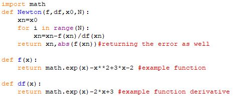
My Newtons Method Code:

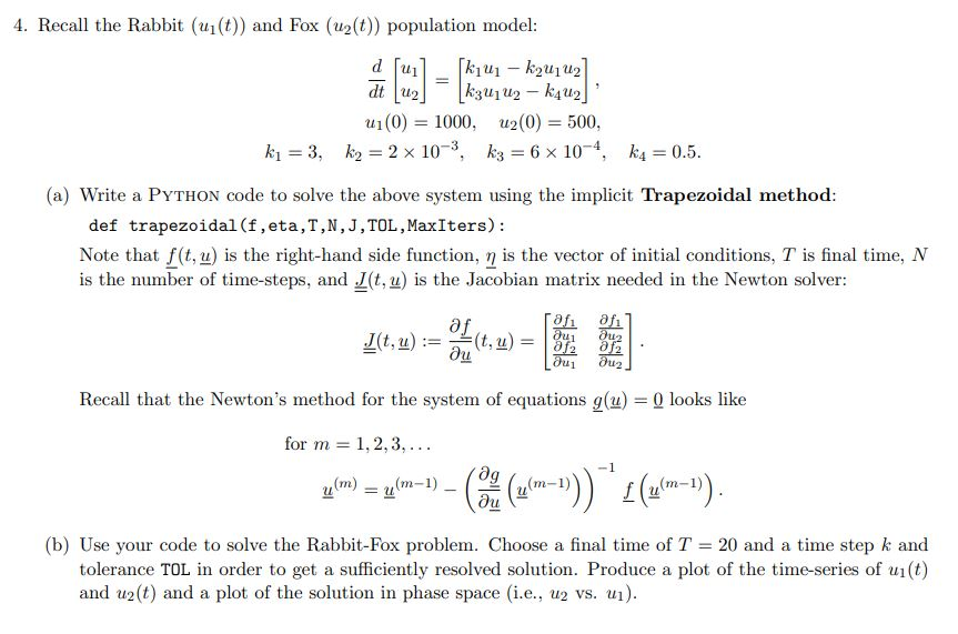
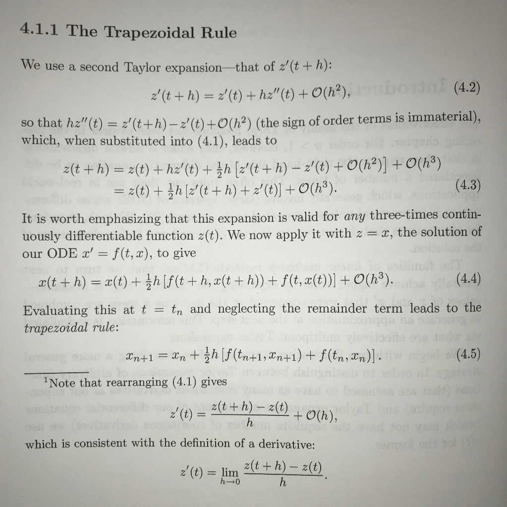
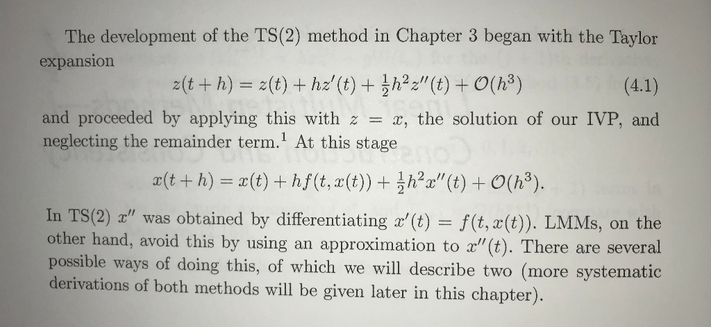
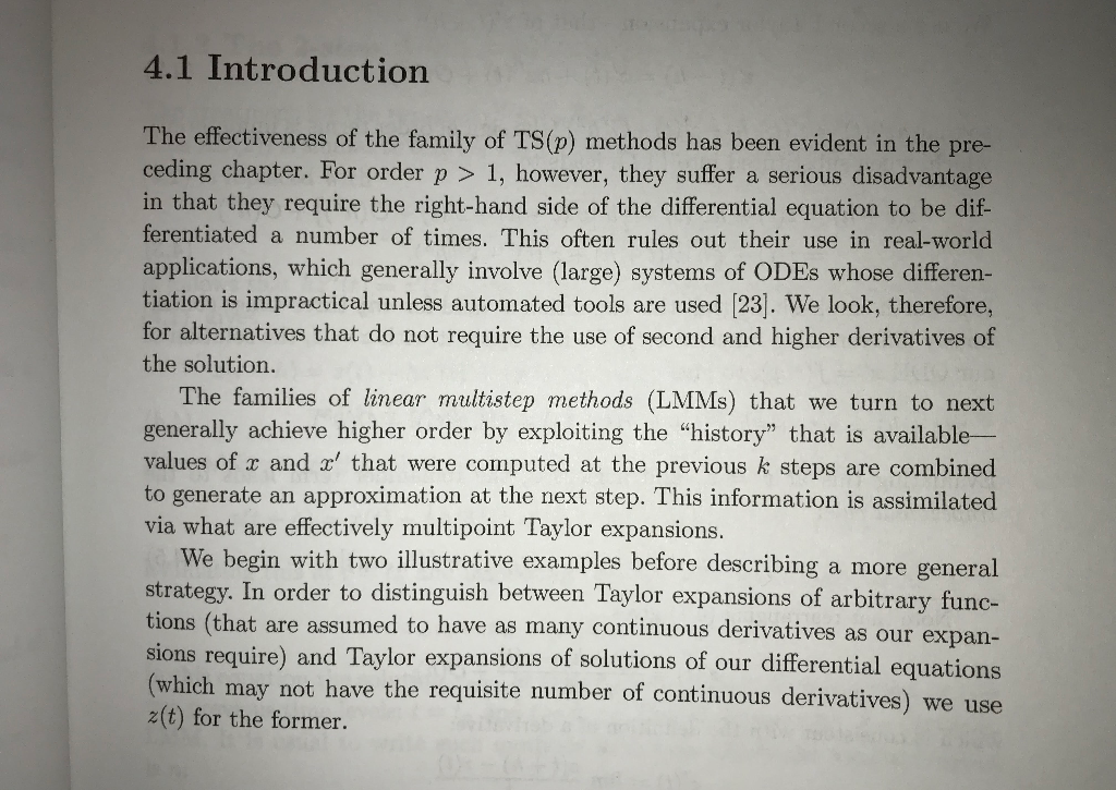
4. Recall the Rabbit (ui(t)) and Fox (uz(t)) population model: d [ui] [k1u1 - k2u1u2] dt [ua] [k3u1 U2 - kauz] u1(0) = 1000, u2(0) = 500, ki = 3, kg = 2 x 10-3, k3 = 6 x 10-4, k4 = 0.5. (a) Write a PYTHON code to solve the above system using the implicit Trapezoidal method: def trapezoidal(f, eta,T,N,J, TOL, MaxIters): Note that f(t, u) is the right-hand side function, n is the vector of initial conditions, T is final time, N is the number of time-steps, and Jit, u) is the Jacobian matrix needed in the Newton solver: rafi afil 214 . 2) = 2) = 2 dui duz Recall that the Newton's method for the system of equations g(u) = 0 looks like for m = 1,2,3,... 2 cm) = y m=1) ((z\m-))) [ (26m-). (b) Use your code to solve the Rabbit-Fox problem. Choose a final time of T = 20 and a time step k and tolerance TOL in order to get a sufficiently resolved solution. Produce a plot of the time-series of uit) and u2(t) and a plot of the solution in phase space (i.e., u2 vs. ui). 4.1.1 The Trapezoidal Rule We use a second Taylor expansionthat of z'(t + h): x' (t+h) = x'(t) + hz"(t) + (ha), bod (4.2) so that hz"(t) = z'(t+h) z' (t)+(92) (the sign of order terms is immaterial), which, when substituted into (4.1), leads to z(t + h) = 2(t) + hz'(t) + 1h [z'(t + h) z'(t) + O(h2)] + O(h3) = z(t) + 3h [z'(t + h) + z'(t)] + O(h3). (4.3) It is worth emphasizing that this expansion is valid for any three-times contin- uously differentiable function z(t). We now apply it with z = x, the solution of our ODE x' = f(t, x), to give | 2(t+h) = x(t) + 3 h (f(t + h, x(t + h)) + f(t, x(t))] + O(hy). (4.4) Evaluating this at t = tn and neglecting the remainder term leads to the trapezoidal rule: som Xn+1 = In + h [f(tn+1, Xn+1) + f(tn, xn)]. w god (4.5) Note that rearranging (4.1) gives bodo bar ) b ' (t) = 2(t+h) z(t) _ ol l which is consistent with the definition of a derivative: 2 (t) = limh (t) = lim &(t +h) - 2(t). The development of the TS(2) method in Chapter 3 began with the Taylor expansion z(t + h) = z(t) + hz'(t) + h2z"(t) + O(h) (4.1) and proceeded by applying this with z = x, the solution of our IVP, and neglecting the remainder term. At this stage x(t + h) = x(t) +hf(t, x(t))+ hx"(t) + O(hy). In TS(2) x" was obtained by differentiating x'(t) = f(t, x(t)). LMMs, on the other hand, avoid this by using an approximation to x"(t). There are several possible ways of doing this, of which we will describe two (more systematic derivations of both methods will be given later in this chapter). 4.1 Introduction The effectiveness of the family of TS(p) methods has been evident in the pre- ceding chapter. For order p > 1, however, they suffer a serious disadvantage in that they require the right-hand side of the differential equation to be dif- ferentiated a number of times. This often rules out their use in real-world applications, which generally involve (large) systems of ODEs whose differen- tiation is impractical unless automated tools are used [23]. We look, therefore, for alternatives that do not require the use of second and higher derivatives of the solution. The families of linear multistep methods (LMMs) that we turn to next generally achieve higher order by exploiting the "history that is available values of x and x' that were computed at the previous k steps are combined to generate an approximation at the next step. This information is assimilated via what are effectively multipoint Taylor expansions. We begin with two illustrative examples before describing a more general strategy. In order to distinguish between Taylor expansions of arbitrary func- tions (that are assumed to have as many continuous derivatives as our expan- sions require) and Taylor expansions of solutions of our differential equations (which may not have the requisite number of continuous derivatives) we use z(t) for the former. the previstory the turn The development of the TS(2) method in Chapter 3 began with the Taylor expansion z(t + h) = z(t) + hz'(t) + h2z"(t) + O(h) (4.1) and proceeded by applying this with z = x, the solution of our IVP, and neglecting the remainder term. At this stage x(t + h) = x(t) +hf(t, x(t))+ hx"(t) + O(hy). In TS(2) x" was obtained by differentiating x'(t) = f(t, x(t)). LMMs, on the other hand, avoid this by using an approximation to x"(t). There are several possible ways of doing this, of which we will describe two (more systematic derivations of both methods will be given later in this chapter). import math def Newton (f, df, x0,N): xn=x0 for i in range (N): xn=xn-f(xn) /df (xn) return xn, abs (f(x)) #returning the error as well def f(x): return math.exp (x) -x**2+3*X-2 #example function def df (x): return math.exp (x) -2*x+3 #example function derivative