

Answered step by step
Verified Expert Solution
Question
1 Approved Answer
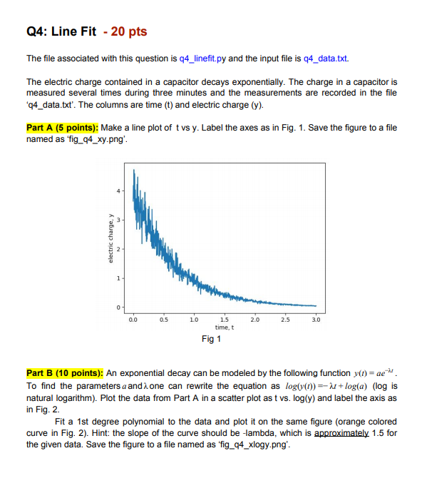
python Q4: Line Fit - 20 pts The file associated with this question is 24_linefit.py and the input file is 04_data.txt. The electric charge contained
 python
Step by Step Solution
There are 3 Steps involved in it
Step: 1

Get Instant Access to Expert-Tailored Solutions
See step-by-step solutions with expert insights and AI powered tools for academic success
Step: 2

Step: 3
Ace Your Homework with AI
Get the answers you need in no time with our AI-driven, step-by-step assistance
Get Started
The Temple Of Django Database Performance
Authors: Andrew Brookins
1st Edition
1734303700, 978-1734303704