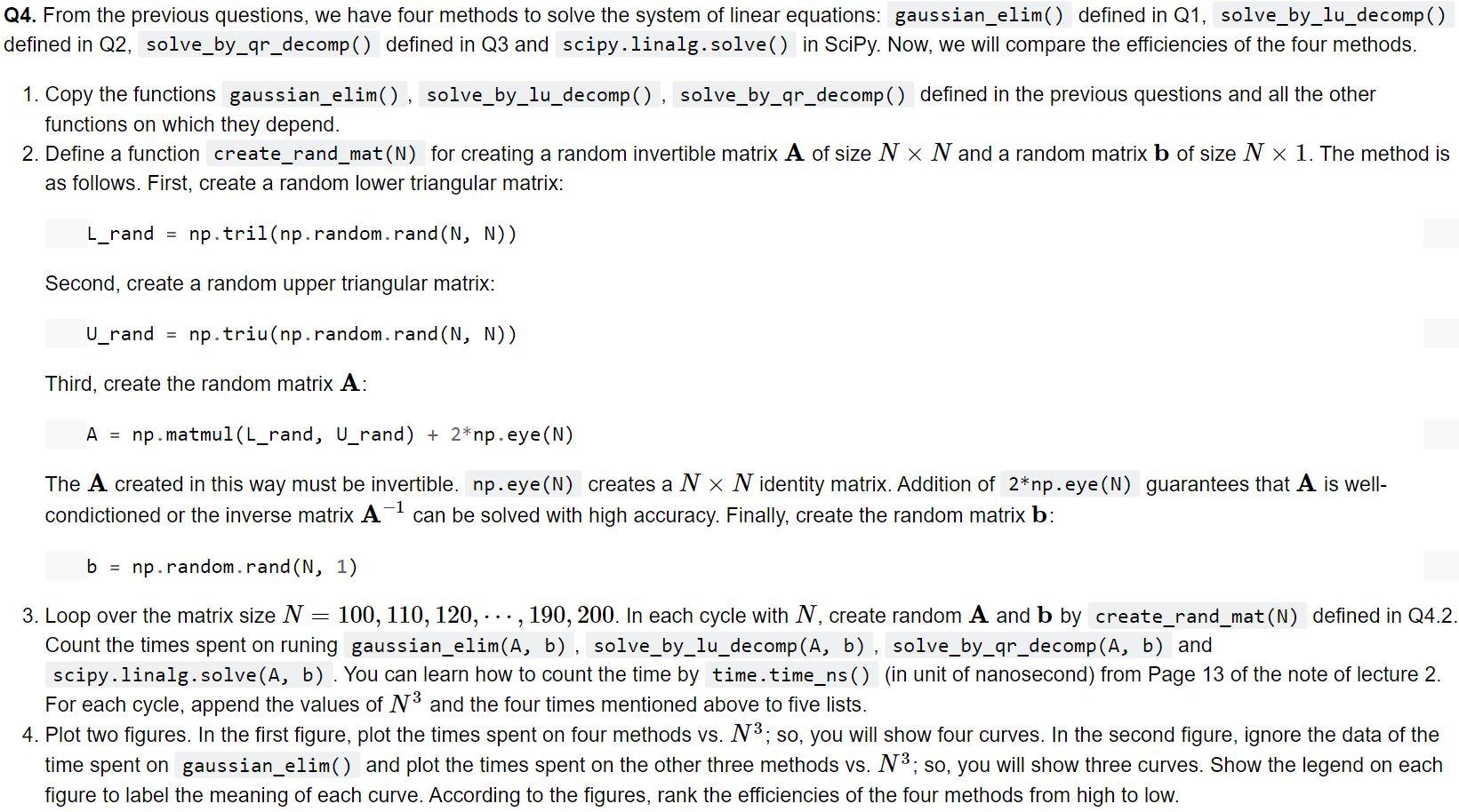
Q4. From the previous questions, we have four methods to solve the system of linear equations: gaussian_elim() defined in Q1, solve_by_lu_decomp() defined in Q2, solve_by_gr_decomp() defined in Q3 and scipy.linalg. solve() in Scipy. Now, we will compare the efficiencies of the four methods. 1. Copy the functions gaussian_elim(), solve_by_lu_decomp() , solve_by_ar_decomp() defined in the previous questions and all the other functions on which they depend. 2. Define a function create_rand_mat(N) for creating a random invertible matrix A of size N ~ N and a random matrix b of size N * 1. The method is as follows. First, create a random lower triangular matrix: L_rand = np. tril(np.random.rand(N, N)) Second, create a random upper triangular matrix: U_rand = np. triu(np.random.rand(N, N)) Third, create the random matrix A: A = np.matmul(L_rand, U_rand) + 2*np.eye(N) The A created in this way must be invertible. np.eye(N) creates a N x N identity matrix. Addition of 2*np.eye(N) guarantees that A is well- condictioned or the inverse matrix A can be solved with high accuracy. Finally, create the random matrix b: b = np.random.rand (N, 1) = 3. Loop over the matrix size N 100, 110, 120,..., 190, 200. In each cycle with N, create random A and b by create_rand_mat(N) defined in Q4.2. Count the times spent on runing gaussian_elim(A, b), solve_by_lu_decomp (A, b), solve_by_gr_decomp (A, b) and scipy.linalg. solve(a, b). You can learn how to count the time by time. time_ns() in unit of nanosecond) from Page 13 of the note of lecture 2. For each cycle, append the values of N3 and the four times mentioned above to five lists. 4. Plot two figures. In the first figure, plot the times spent on four methods vs. N3; so, you will show four curves. In the second figure, ignore the data of the time spent on gaussian_elim() and plot the times spent on the other three methods vs. N3; so, you will show three curves. Show the legend on each figure to label the meaning of each curve. According to the figures, rank the efficiencies of the four methods from high to low. Q4. From the previous questions, we have four methods to solve the system of linear equations: gaussian_elim() defined in Q1, solve_by_lu_decomp() defined in Q2, solve_by_gr_decomp() defined in Q3 and scipy.linalg. solve() in Scipy. Now, we will compare the efficiencies of the four methods. 1. Copy the functions gaussian_elim(), solve_by_lu_decomp() , solve_by_ar_decomp() defined in the previous questions and all the other functions on which they depend. 2. Define a function create_rand_mat(N) for creating a random invertible matrix A of size N ~ N and a random matrix b of size N * 1. The method is as follows. First, create a random lower triangular matrix: L_rand = np. tril(np.random.rand(N, N)) Second, create a random upper triangular matrix: U_rand = np. triu(np.random.rand(N, N)) Third, create the random matrix A: A = np.matmul(L_rand, U_rand) + 2*np.eye(N) The A created in this way must be invertible. np.eye(N) creates a N x N identity matrix. Addition of 2*np.eye(N) guarantees that A is well- condictioned or the inverse matrix A can be solved with high accuracy. Finally, create the random matrix b: b = np.random.rand (N, 1) = 3. Loop over the matrix size N 100, 110, 120,..., 190, 200. In each cycle with N, create random A and b by create_rand_mat(N) defined in Q4.2. Count the times spent on runing gaussian_elim(A, b), solve_by_lu_decomp (A, b), solve_by_gr_decomp (A, b) and scipy.linalg. solve(a, b). You can learn how to count the time by time. time_ns() in unit of nanosecond) from Page 13 of the note of lecture 2. For each cycle, append the values of N3 and the four times mentioned above to five lists. 4. Plot two figures. In the first figure, plot the times spent on four methods vs. N3; so, you will show four curves. In the second figure, ignore the data of the time spent on gaussian_elim() and plot the times spent on the other three methods vs. N3; so, you will show three curves. Show the legend on each figure to label the meaning of each curve. According to the figures, rank the efficiencies of the four methods from high to low


