qt(0.95,df=292)

[1] 1.650089

qt(0.975,df=292)

[1] 1.968121

qf(0.95,df1=1,df2=292)

[1] 3.873502

qf(0.95,df1=292,df2=293)

[1] 1.212453

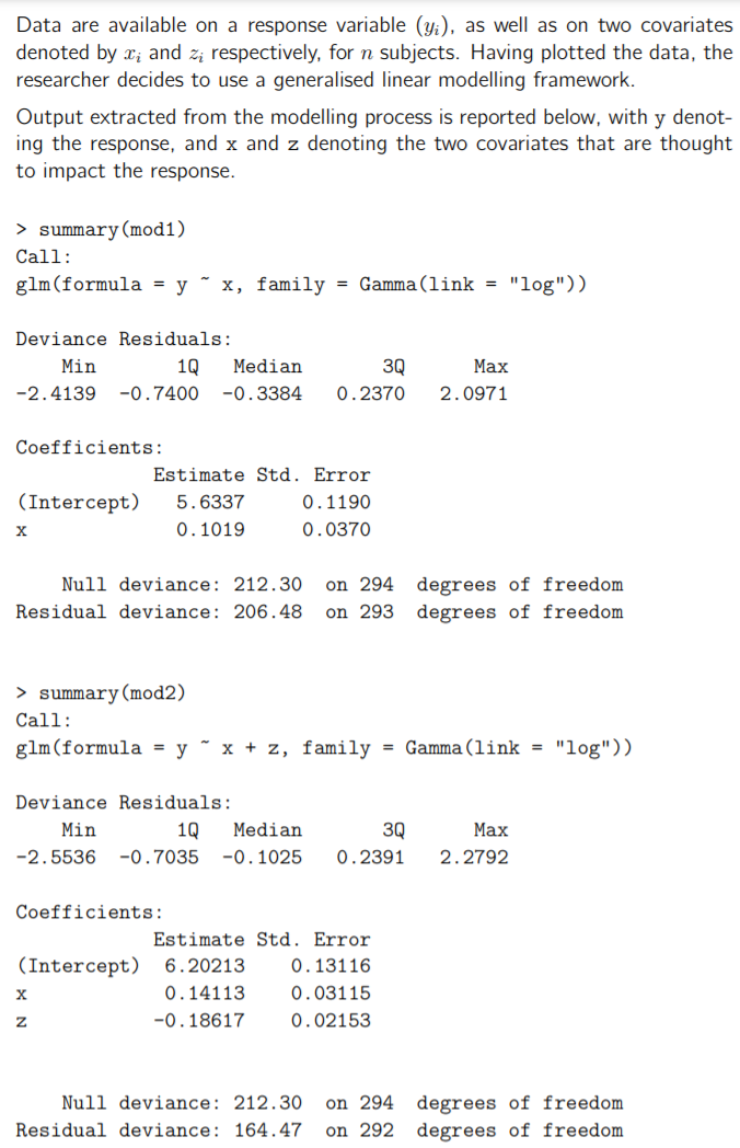
(a) Construct an analysis of deviance to decide which of the models mod1 or mod2 should be preferred at the significance level 5%. Clearly justify your model choice through stating the tested hypotheses, the test statistic and its distribution and state your conclusion.

(b) Define the Pearson residuals and estimate their approximate mean and variance, under the assumption that model mod2 fits the data. Under model mod2 compute the Pearson residual for the 100th observation, given that it has covariate values x=2 and z=5, and response y=568.

(c) How would you employ kernel density estimation to verify whether the distribution of the deviance residuals indicates a good model fit? Propose a kernel-based density estimator for their density function and show that your proposed estimator satisfies the density function conditions. Explain the impact of bandwidth choice on the density estimator.

(d) Replace mod1 by a new model, say modNR, which is specified using a nonparametric regression framework. Clearly (i) define modNR, (ii) contrast it with mod1, and (iii) outline the principle of local polynomial estimation (without undertaking any derivations).

(e) Carefully explain (i) the impact of the choice of kernel and bandwidth on the local polynomial estimator and (ii) the cross-validation criterion for bandwidth selection for the standard univariate nonparametric regression model.

Data are available on a response variable (yi), as well as on two covariates denoted by X; and zi respectively, for n subjects. Having plotted the data, the researcher decides to use a generalised linear modelling framework. Output extracted from the modelling process is reported below, with y denot- ing the response, and x and z denoting the two covariates that are thought to impact the response. > summary (mod1) Call: glm(formula = y x, family = Gamma (link = "log")) Deviance Residuals: Min 1Q Median -2.4139 -0.7400 -0.3384 30 0.2370 Max 2.0971 Coefficients: Estimate Std. Error (Intercept) 5.6337 0.1190 0.1019 0.0370 Null deviance: 212.30 Residual deviance: 206.48 on 294 degrees of freedom on 293 degrees of freedom > summary (mod2) Call: glm(formula = y^x + z, family = Gamma (link = "log")) Deviance Residuals: Min 1Q Median -2.5536 -0.7035 -0.1025 3Q 0.2391 Max 2.2792 Coefficients: Estimate Std. Error (Intercept) 6.20213 0.13116 X 0.14113 0.03115 Z -0.18617 0.02153 Null deviance: 212.30 Residual deviance: 164.47 on 294 degrees of freedom on 292 degrees of freedom