QUESTION 1:
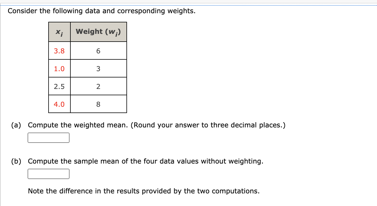
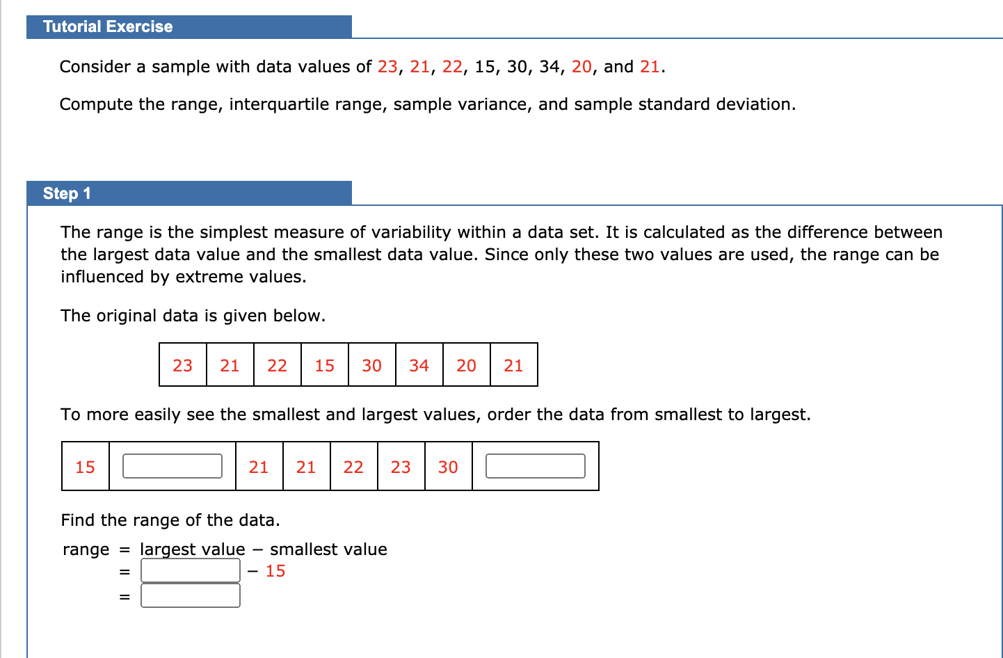
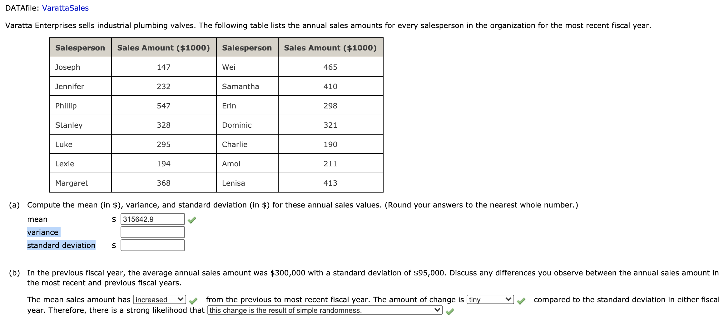
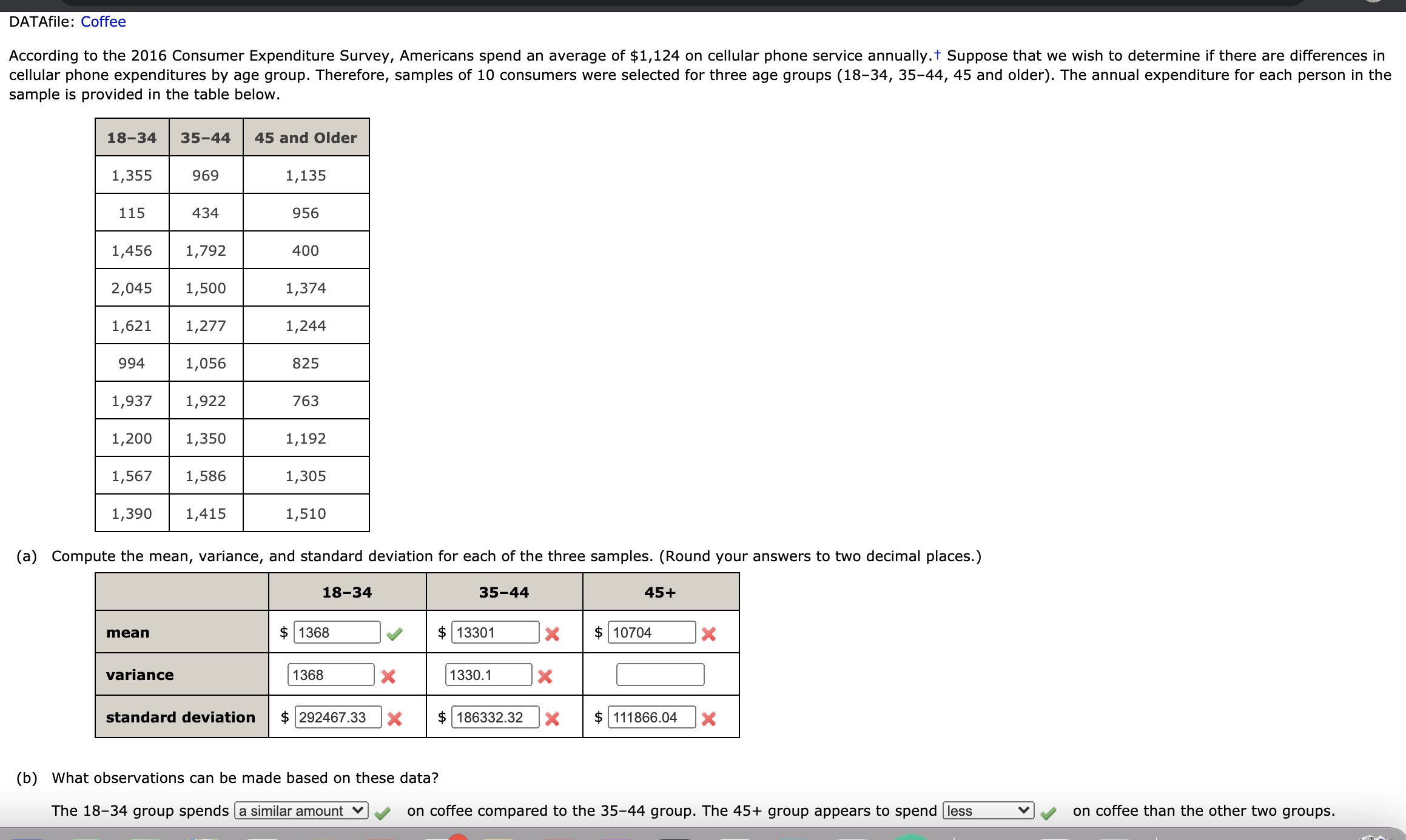
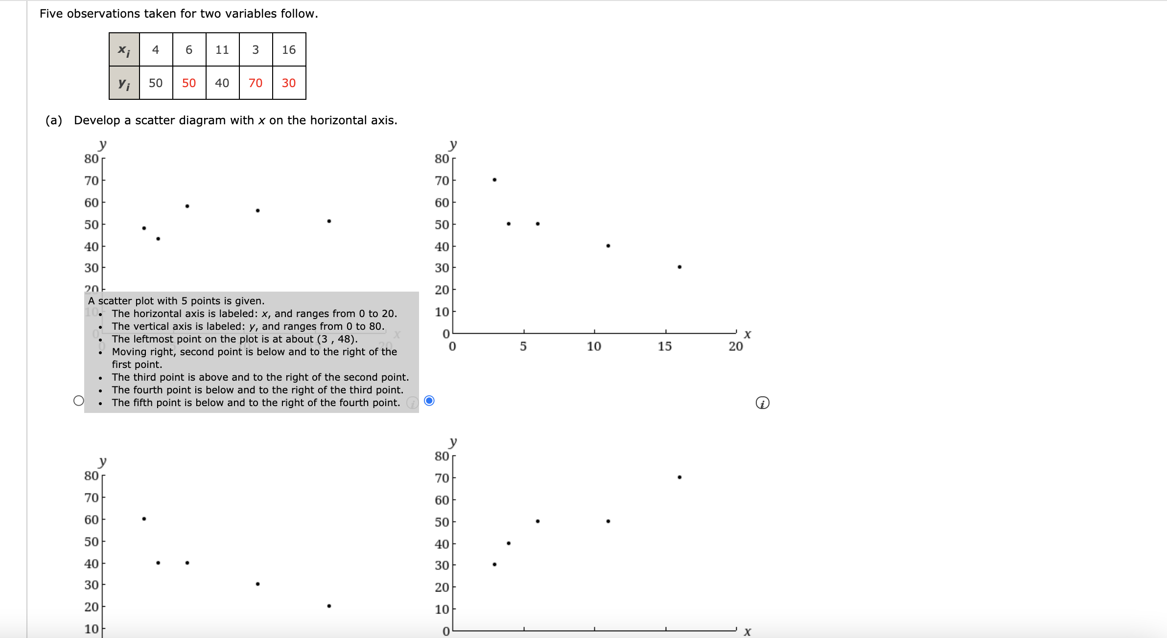
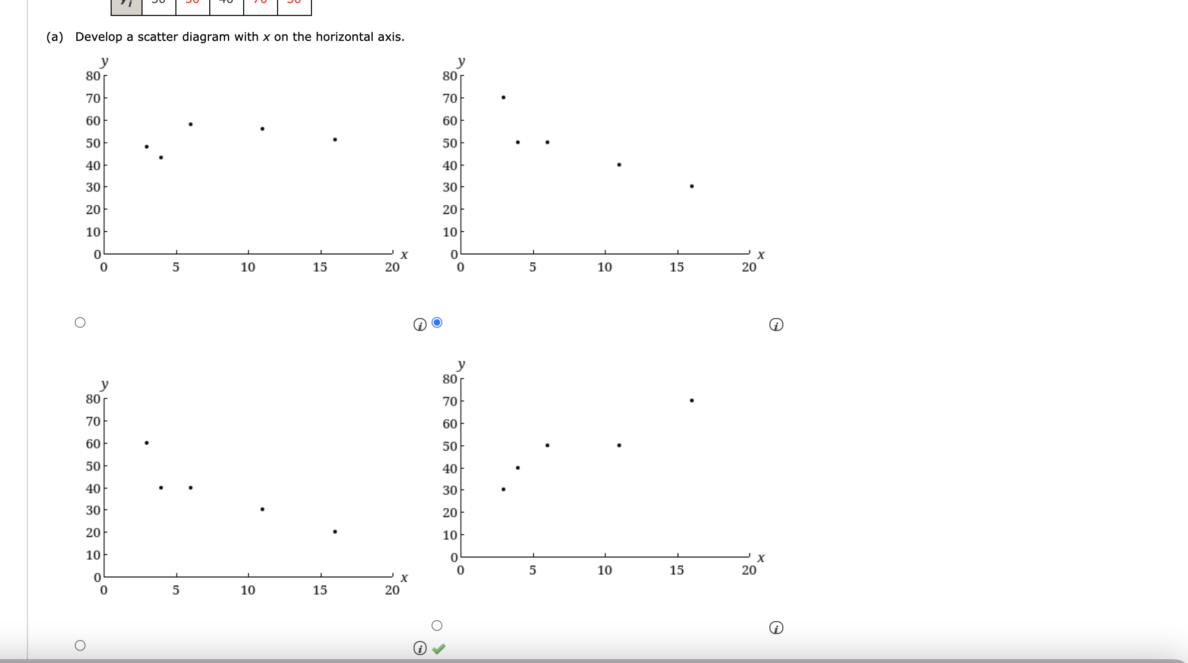
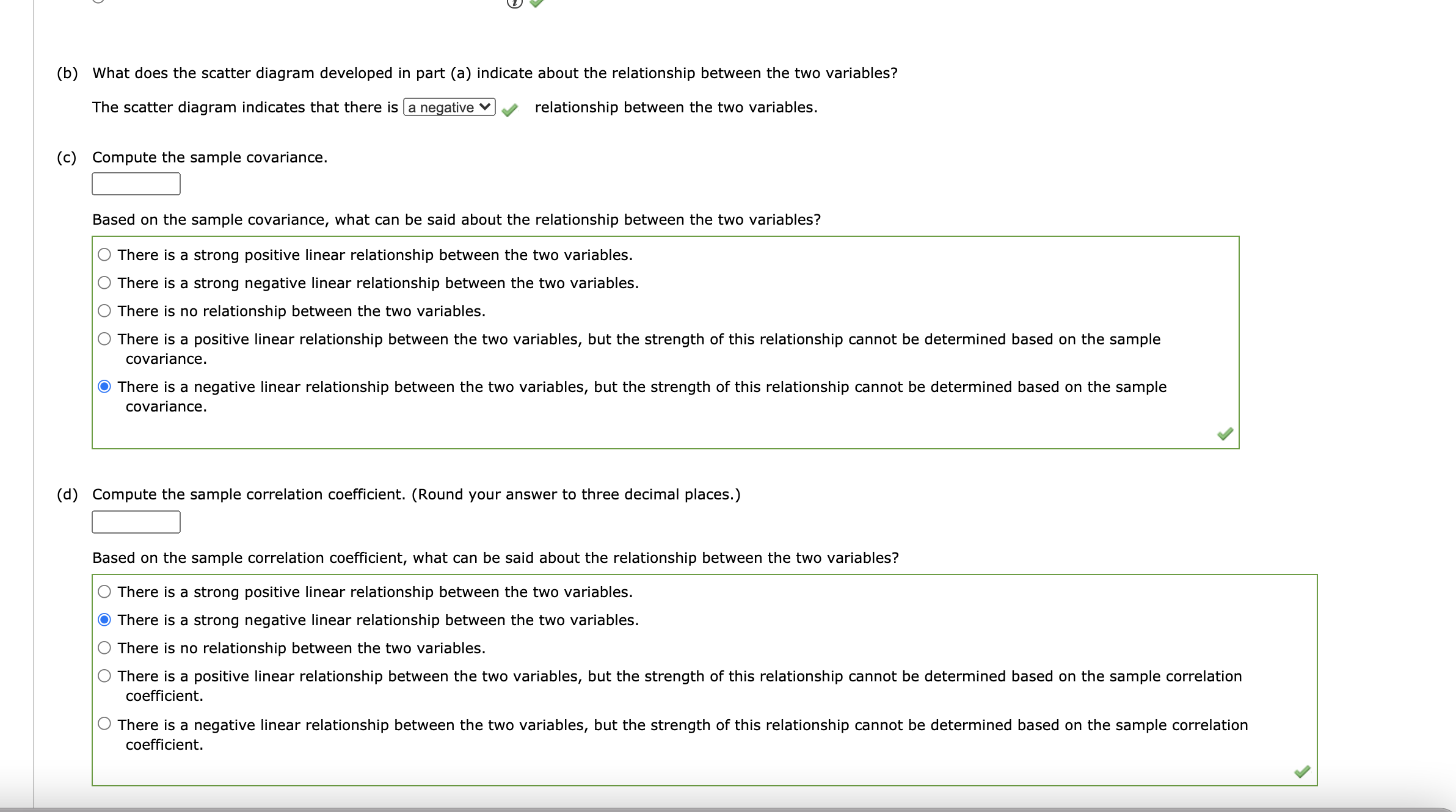
(a) Compute the weighted mean. (Round your answer to three decimal places.) |:| (b) Compute the sample mean of the four data values without weighting. Note the difference in the results provided by the two computations. Tutorial Exercise Consider a sample with data values of 23, 21, 22, 15, 30, 34, 20, and 21. Compute the range, interquartile range, sample variance, and sample standard deviation. Step 1 The range is the simplest measure of variability within a data set. It is calculated as the difference between the largest data value and the smallest data value. Since only these two values are used, the range can be influenced by extreme values. The original data is given below. 23 21 22 15 30 34 20 21 To more easily see the smallest and largest values, order the data from smallest to largest. 15 21 21 22 23 30 Find the range of the data. range = largest value - smallest value - 15DATAfile: VarattaSales Varatta Enterprises sells industrial plumbing valves. The following table lists the annual sales amounts for every salesperson in the organization for the most recent fiscal year. Salesperson Sales Amount ($1000) Salesperson Sales Amount ($1000) Joseph 147 Wei 465 Jennifer 232 Samantha 410 Phillip 547 Erin 298 Stanley 328 Dominic 321 Luke 295 Charlie 190 Lexie 194 Amol 211 Margaret 368 Lenisa 413 (a) Compute the mean (in $), variance, and standard deviation (in $) for these annual sales values. (Round your answers to the nearest whole number.) mean $ 315642.9 variance standard deviation $ (b) In the previous fiscal year, the average annual sales amount was $300,000 with a standard deviation of $95,000. Discuss any differences you observe between the annual sales amount in the most recent and previous fiscal years. The mean sales amount has increased | from the previous to most recent fiscal year. The amount of change is tiny v compared to the standard deviation in either fiscal year. Therefore, there is a strong likelihood that this change is the result of simple randomness.DATAfile: Coffee According to the 2016 Consumer Expenditure Survey, Americans spend an average of $1,124 on cellular phone service annually. Suppose that we wish to determine if there are differences in cellular phone expenditures by age group. Therefore, samples of 10 consumers were selected for three age groups (18-34, 35-44, 45 and older). The annual expenditure for each person in the sample is provided in the table below. 18-34 35-44 45 and Older 1,355 969 1,135 115 434 956 1,456 1,792 400 2,045 1,500 1,374 1,621 1,277 1,244 994 1,056 825 1,937 1,922 763 1,200 1,350 1, 192 1,567 1,586 1,305 1,390 1,415 1,510 (a) Compute the mean, variance, and standard deviation for each of the three samples. (Round your answers to two decimal places.) 18-34 35-44 45+ mean $ 1368 $ 13301 X $ 10704 X variance 1368 X 1330.1 X standard deviation $ 292467.33 X $ 186332.32 X $ 111866.04 X (b) What observations can be made based on these data? The 18-34 group spends |a similar amount v on coffee compared to the 35-44 group. The 45+ group appears to spend less v on coffee than the other two groups.Consider a sample with a mean of 500 and a standard deviation of 100. What are the z-scores for the following data values: 520, 680, 500, 440, and 270? z-score for 520 z-score for 680 z-score for 500 z-score for 440 z-score for 270Suppose that the mean retail price per gallon of regular grade gasoline in the United States is $3.47 with a standard deviation of $0.20 and that the retail price per gallon has a bell-shaped distribution. (a) What percentage of regular grade gasoline sold between $3.27 and $3.67 per gallon? 12 x % (b) What percentage of regular grade gasoline sold between $3.27 and $3.87 per gallon? % (c) What percentage of regular grade gasoline sold for more than $3.87 per gallon? % Five observations taken for two variables follow. X; 6 1 1 3 16 yi 50 50 40 70 30 (a) Develop a scatter diagram with x on the horizontal axis. y 80 y 80 70 70 60 60 50 50- 40 40 30 30 A scatter plot with 5 points is given. 20 The horizontal axis is labeled: x, and ranges from 0 to 20. 10/ The vertical axis is labeled: y, and ranges from 0 to 80. The leftmost point on the plot is at about (3 , 48). Moving right, second point is below and to the right of the 5 X 10 15 20 first point. The third point is above and to the right of the second point. The fourth point is below and to the right of the third point. The fifth point is below and to the right of the fourth point. O y 80 80 70 70 60 60 50 50 40 40 30 30 20 20 10/ 10 0\f(b) What does the scatter diagram developed in part (a) indicate about the relationship between the two variables? The scatter diagram indicates that there is a negative v y relationship between the two variables. (c) Compute the sample covariance. Based on the sample covariance, what can be said about the relationship between the two variables? 0 There is a strong positive linear relationship between the two variables. 0 There is a strong negative linear relationship between the two variables. 0 There is no relationship between the two variables. 0 There is a positive linear relationship between the two variables, but the strength of this relationship cannot be determined based on the sample covariance. There is a negative linear relationship between the two variables, but the strength of this relationship cannot be determined based on the sample covariance. (d) Compute the sample correlation coefcient. (Round your answer to three decimal places.) Based on the sample correlation coefficient, what can be said about the relationship between the two variables? 0 There is a strong positive linear relationship between the two variables. There is a strong negative linear relationship between the two variables. 0 There is no relationship between the two variables. 0 There is a positive linear relationship between the two variables, but the strength of this relationship cannot be determined based on the sample correlation coefcient. 0 There is a negative linear relationship between the two variables, but the strength of this relationship cannot be determined based on the sample correlation coefcient
