Question 1

Enter the company name Luxury Chairs by [YOUR NAME] in cell B2. Format to be Title format. Format B3 to be Heading 4.

Use an appropriate function to enter the current date in cell I2.

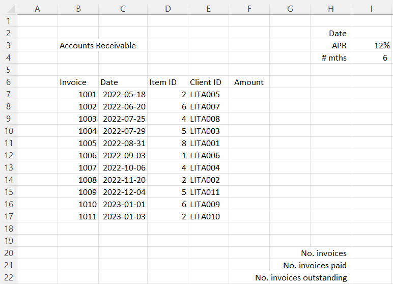
In cell F7, use an appropriate function to show the price for the item sold to the client, using the price data found on the Data worksheet (cells B3:D14). Copy this formula to all rows of data.

Add a new column header in cell G6 called Monthly Payment. In cell G7, use an appropriate finance function to calculate the monthly payment using the APR and # months in cells I3:I4. Set the PV as a negative to have your resulting payment amount show as a positive number. Copy this formula to all rows of data.

Add a new column header in cell H6 called Final Payment Date. In cell H7, use an appropriate date function to show the date of the final payment, based on the sale date in cell C7 and the number of months of the company's financing plan in cell I4. Remember, the first payment is made on the sale date (so it counts as the first of 6 total payments). Copy this formula to all data rows.

Format all dates (columns C and H of the data and cell I2) to show as dd-mmm-yy.

Add a new column header in cell I6 called Fully Paid. In cell I7, create an IF statement to display "YES" if the purchase is fully paid or "NO" if the final payment date is still in the future (based on the final payment date in cell H7 and the current date in cell I2). Copy formula to all data rows.

Let's format:

Format the sales price data in column F to be accounting, no decimals and the monthly payment data in column G to be accounting, 2 decimals.

Centre data in columns B, D, E and I.

Wrap and centre all headers in row 6 and set all column widths B:I to 10.

Set the theme of this worksheet to Parcel and change the colours to Slipstream.

Fill the header row 6 to light blue, background 2 (top row). Add a thick bottom border. Apply bold font.

SUM the amount in cell F18, formatted as accounting zero decimals. Show the AVERAGE monthly payment in cell G18, formatted as accounting 2 decimals. Apply a single top and double bottom border for both.

(NEED IN EXCEL FILE)

No. invoices No. invoices paid No. invoices outstanding