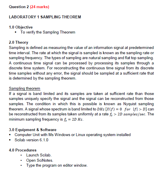
Question $2(24$ marks$)$

LABORATORY $1$ SAMPLING THEOREM

$1\mathrm{.}0$ Objective

To verify the Sampling Theorem

$2\mathrm{.}0$ Theory

Sampling is defined as measuring the value of an information signal at predetermined

time interval. The rate at which the signal is sampled is known as the sampling rate or

sampling frequency. The types of sampling are natural sampling and flat top sampling.

A continuous time signal can be processed by processing its samples through a

discrete time system. For reconstructing the continuous time signal from its discrete

time samples without any error, the signal should be sampled at a sufficient rate that

is determined by the sampling theorem.

Sampling theorem

If a signal is band limited and its samples are taken at sufficient rate than those

samples uniquely specify the signal and the signal can be reconstructed from those

samples. The condition in which this is possible is known as Nyquist sampling

theorem. A signal whose spectrum is band limited to for $|f|>D$ can

be reconstructed from its samples taken uniformly at a rate $f_s>2D$ samples $\frac{?}{sec}.$ The

minimum sampling frequency is $f_s=2DHz.$

$3\mathrm{.}0$ Equipment & Software

Computer Unit with Ms Windows or Linux operating system installed

Scilab version $6\mathrm{.}1\mathrm{.}0$

$4\mathrm{.}0$ Procedures

Launch Scilab.

Open SciNotes.

Type the program on editor window. Source Code:close;

clear;

fm$=$input$(\text{'}$Enter the input signal frequency:$\text{'})$;

k$=$inout$(\text{'}$Enter the number of Cycles of input signal:$\text{'})$;

A$=$inout$(\text{'}$Enter the amplitude of input signal:$\text{'})$;

tm$=0$:$1/($fm$*$fm$)$:k$/$fm;

x$\}=\backslash$mp@subsup$\{\backslash$textrm$\{$A$\}\}\{\}\{\%\backslash$mp@subsup$\{\backslash$mathrm$\{$ pi$\}\}\{\}\{*\}\backslash$textrm$\{$fm

figure$(1)$;

a $=$ gca$()$;

a$.$x$\_$location $=$ "origin";

a$.$y$\_$location $=$ "origin";

plot$($tm$,$x$)$;

title$(\text{'}$ORIGINAL SIGNAL'$)$;

xlabel$(\text{'}$Time$\text{'})$;

ylabel$(\text{'}$Amplitude$\text{'})$;

Xgrid$(1)$

$//$Sampling Rate$($Nyquist Rate$)=2*$fm

fnyq$=2*$fm;

$.$ UNDER SAMPLING fs$=(3/4)$

a $=$ gca$()$;

a$.$x$\_$location $=$ "origin"; a$.$y$\_$location $=$ "origin"; plot$2$d$3(\text{'}$gnn$\text{'},$n$,$xn$)$; plot$($n$,$xn$,\text{'}$r$\text{'})$; title$(\text{'}$Under

Sampling'$)$; xlabel$(\text{'}$Time$\text{'})$; ylabel$(\text{'}$Amplitude$\text{'})$;

legend$(\text{'}$Sampled Signal', 'Reconstructed Signal'$)$; xgrid$(1)$

$//$NYQUIST SAMPLING fs$=$fnyq; n$=0$:$1/$fs k$/$fm; xn$=$A$*\}\backslash$operatorname$\{$cos$(2*\%$pin$)$; figure$(3)$;

a $=$ gca$()$;

a$.$x$\_$location $=$ "origin"; a$.$y$\_$location $=$ "origin"; plot$2$d$3(\text{'}$gnn$\text{'},$n$,$xn$)$; plot$($n$,$xn$,\text{'}$r$\text{'})$; title$(\text{'}$Nyquist

Sampling'$)$; xlabel$(\text{'}$Time$\text{'})$; ylabel$(\text{'}$Amplitude$\text{'})$;

leqend$(\text{'}$Sampled Signal', 'Reconstructed Signal'$)$; xgrid$(1)$

$//$OVER SAMPLING fs$=$fnyq$\}\backslash$operatorname$\{$cos$(2*\%$pin$)$; figure$(4)$;

a $=$ gca$()$;

a$.$x$\_$location $=$ "origin"; a$.$y$\_$location $=$ "origin"; plot$2$d$3(\text{'}$gnn$\text{'},$n$,$xn$)$; plot$($n$,$xn$,\text{'}$r$\text{'})$;title$(\text{'}$Over

Sampling'$)$; xlabel$(\text{'}$Time$\text{'})$; ylabel$(\text{'}$Amplitude$\text{'})$;

legend$(\text{'}$Sampled Signal', 'Reconstructed Signal'$)$; xgrid$(1)$Sample inputs:

$//$Enter the input signal frequency:$100$

$//$Enter the number of Cycles of input signal:$2$

$//$Enter the amplitude of input signal:$2$

Save the program with filename $.$sce extension.

Execute the program and observe the output or waveforms.