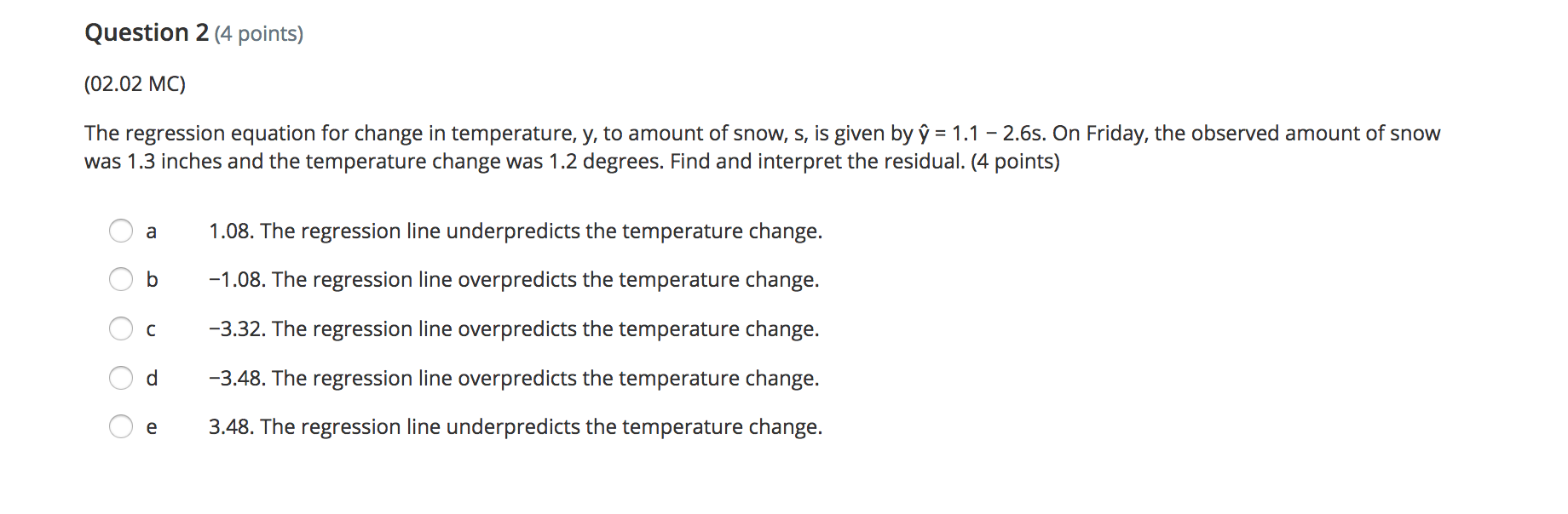
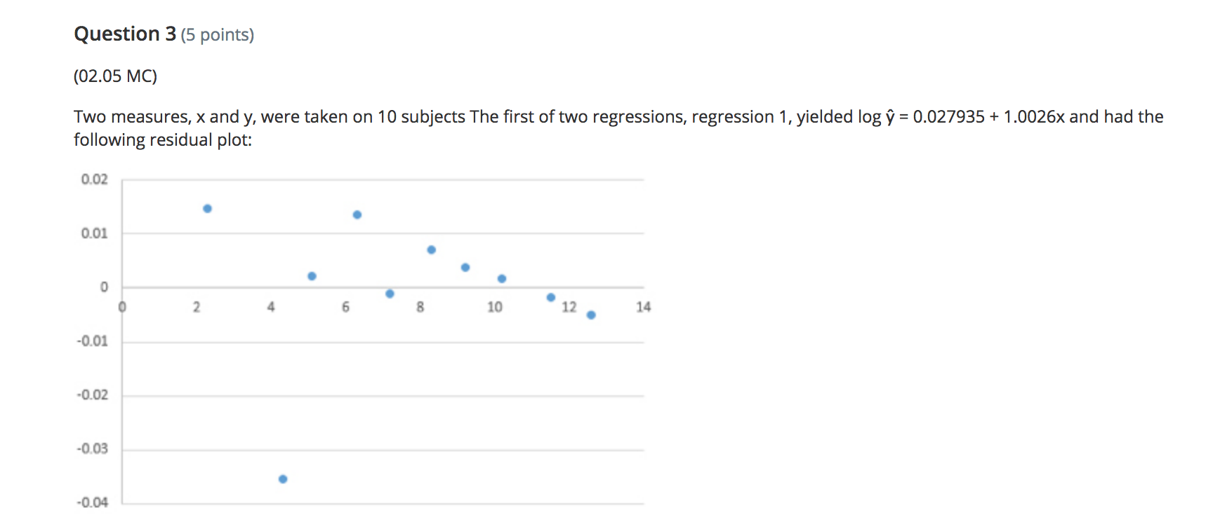
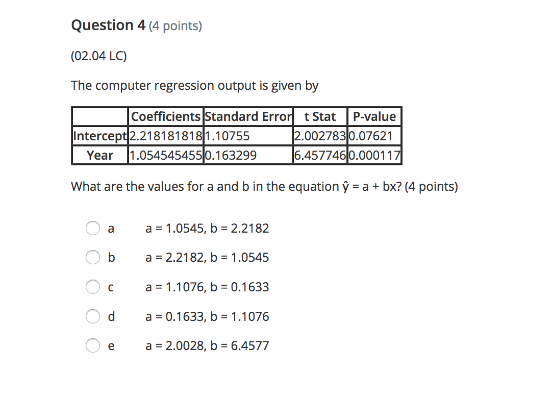
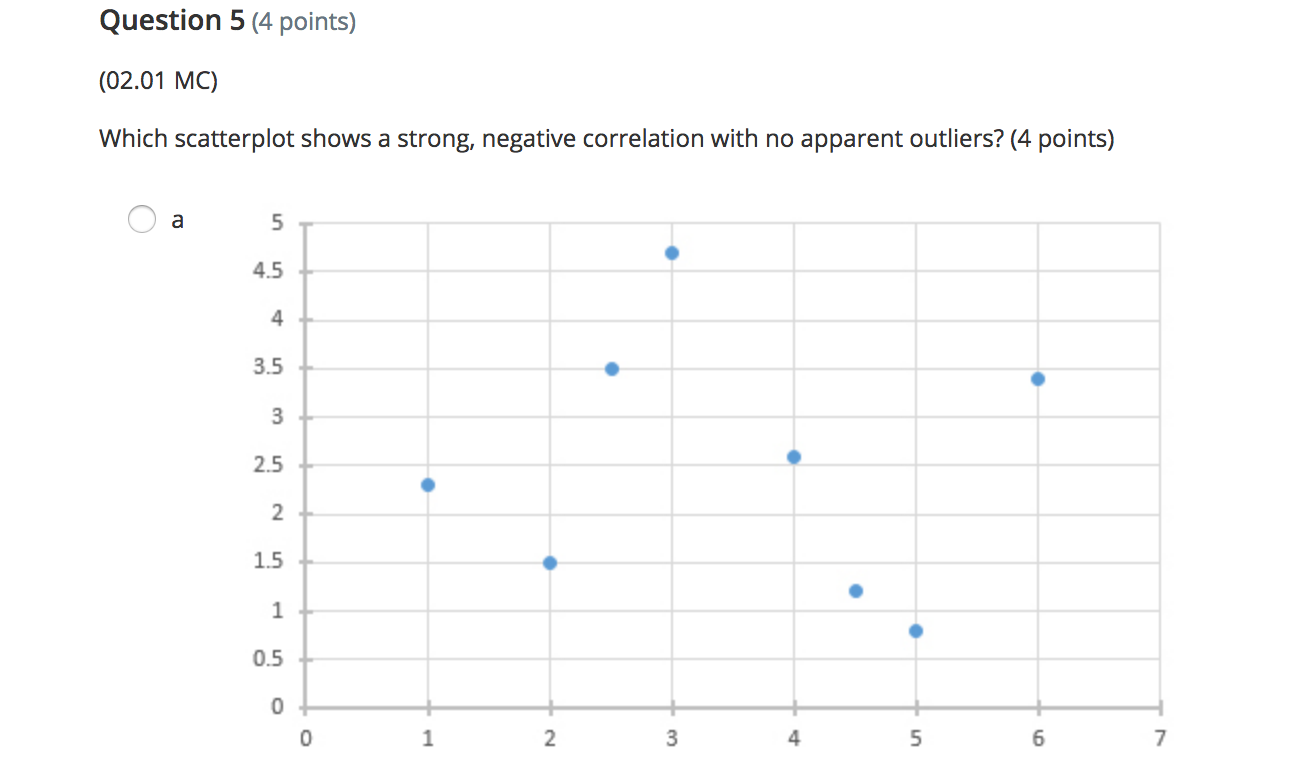
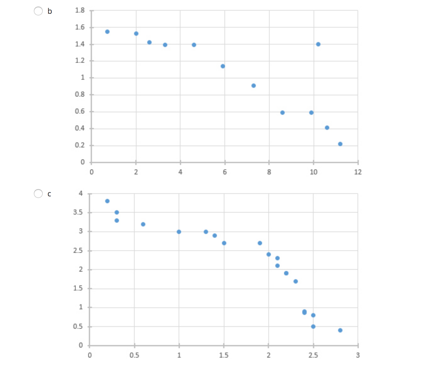
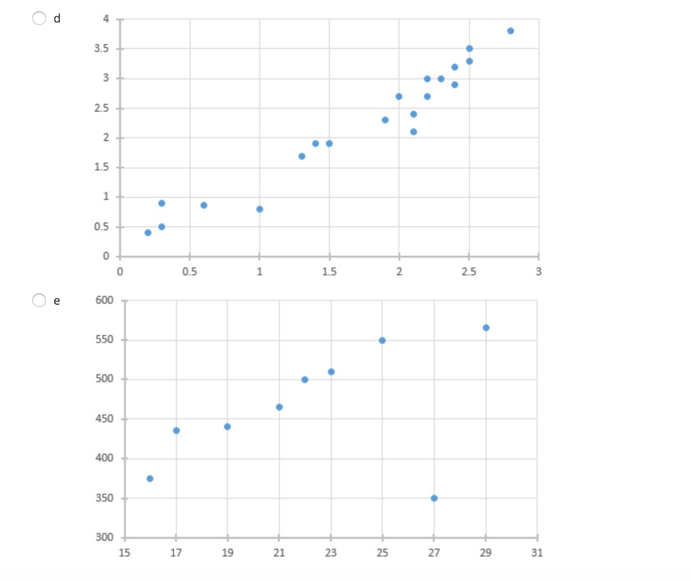
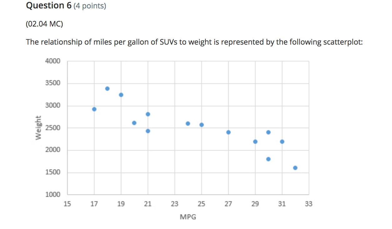
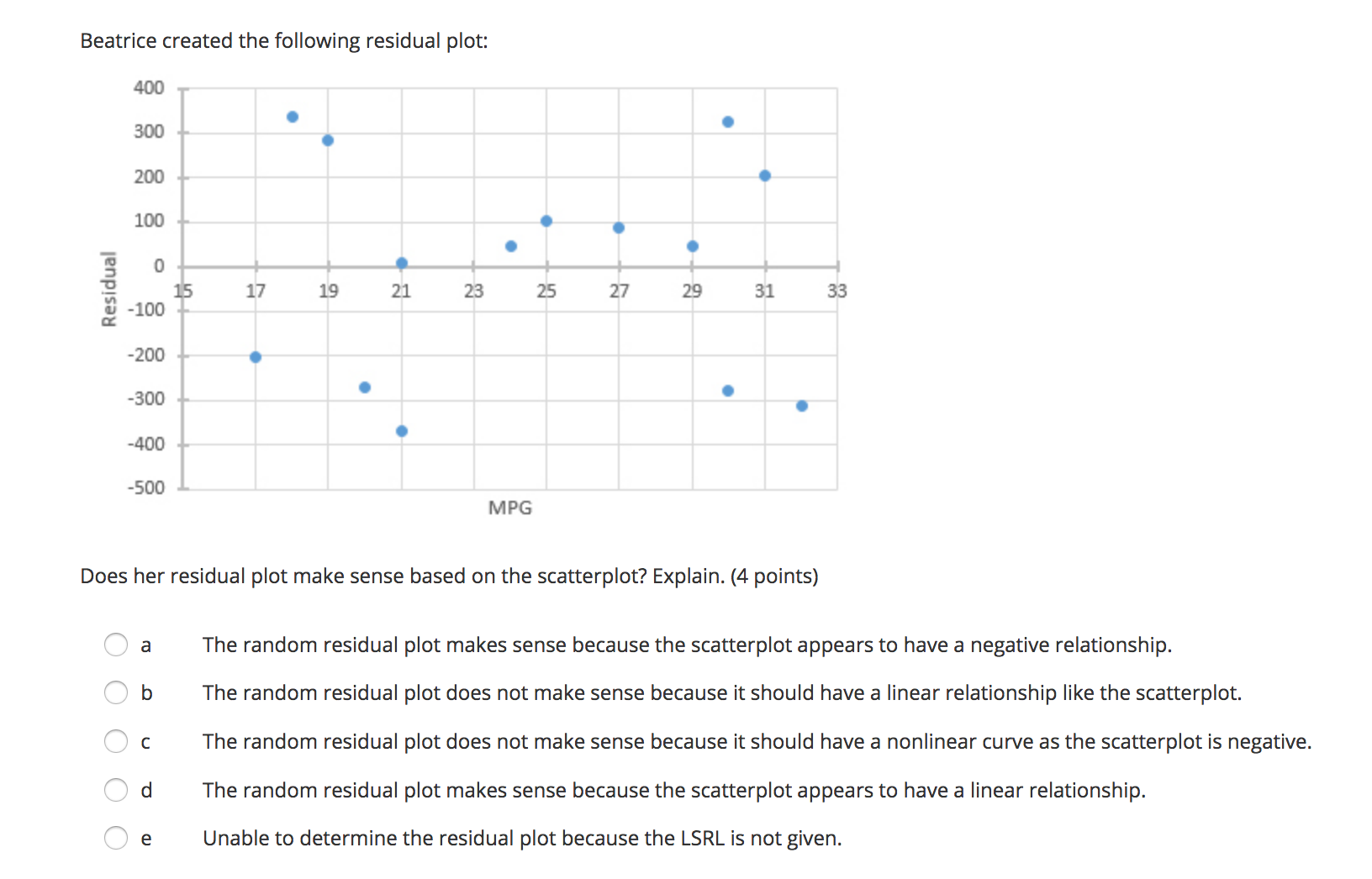
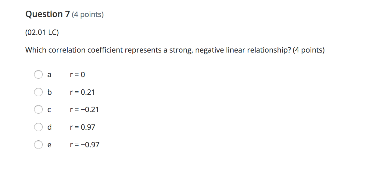
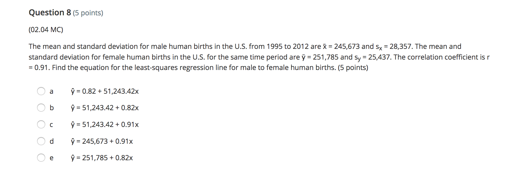
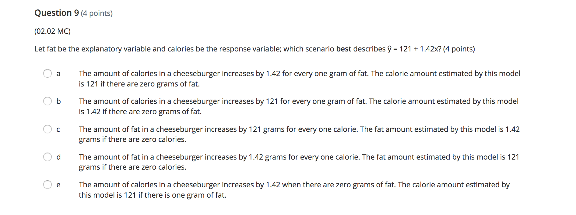
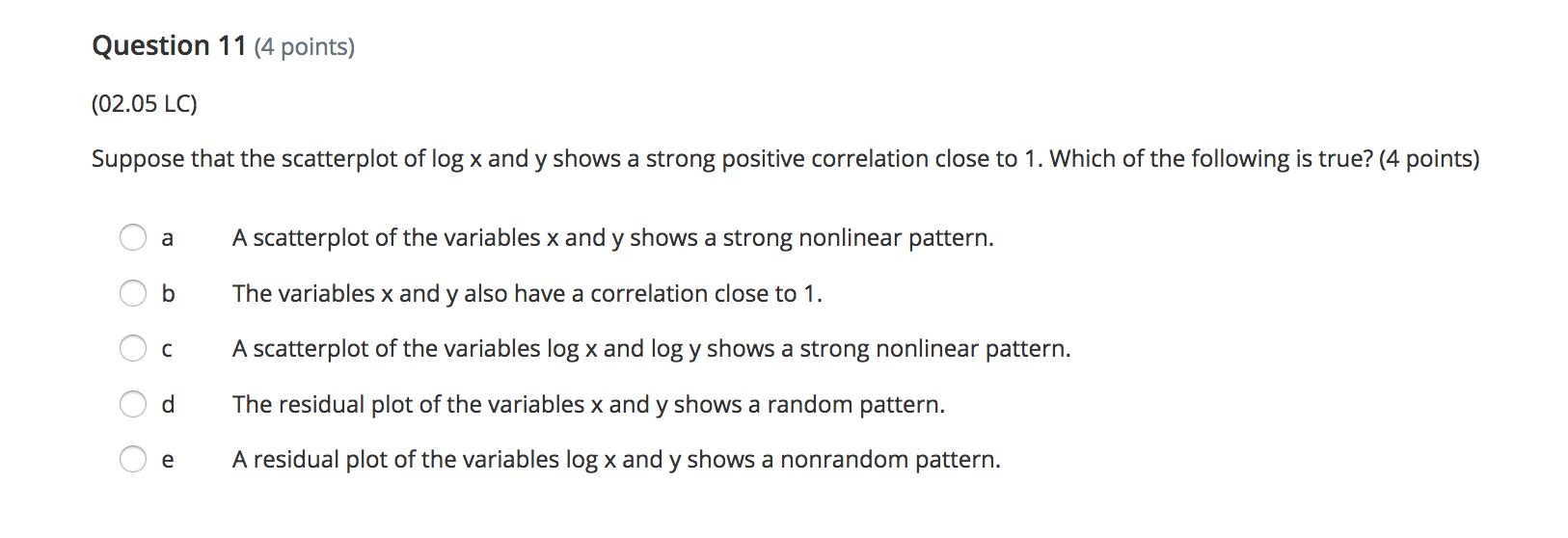
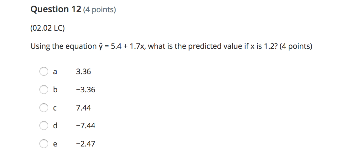
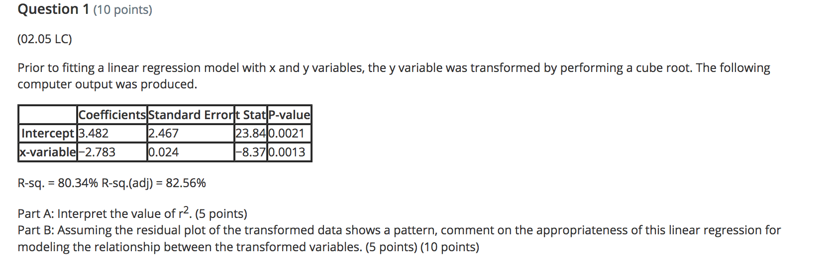
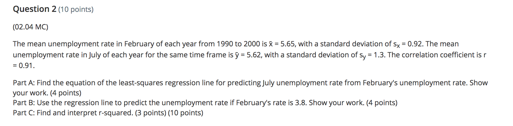
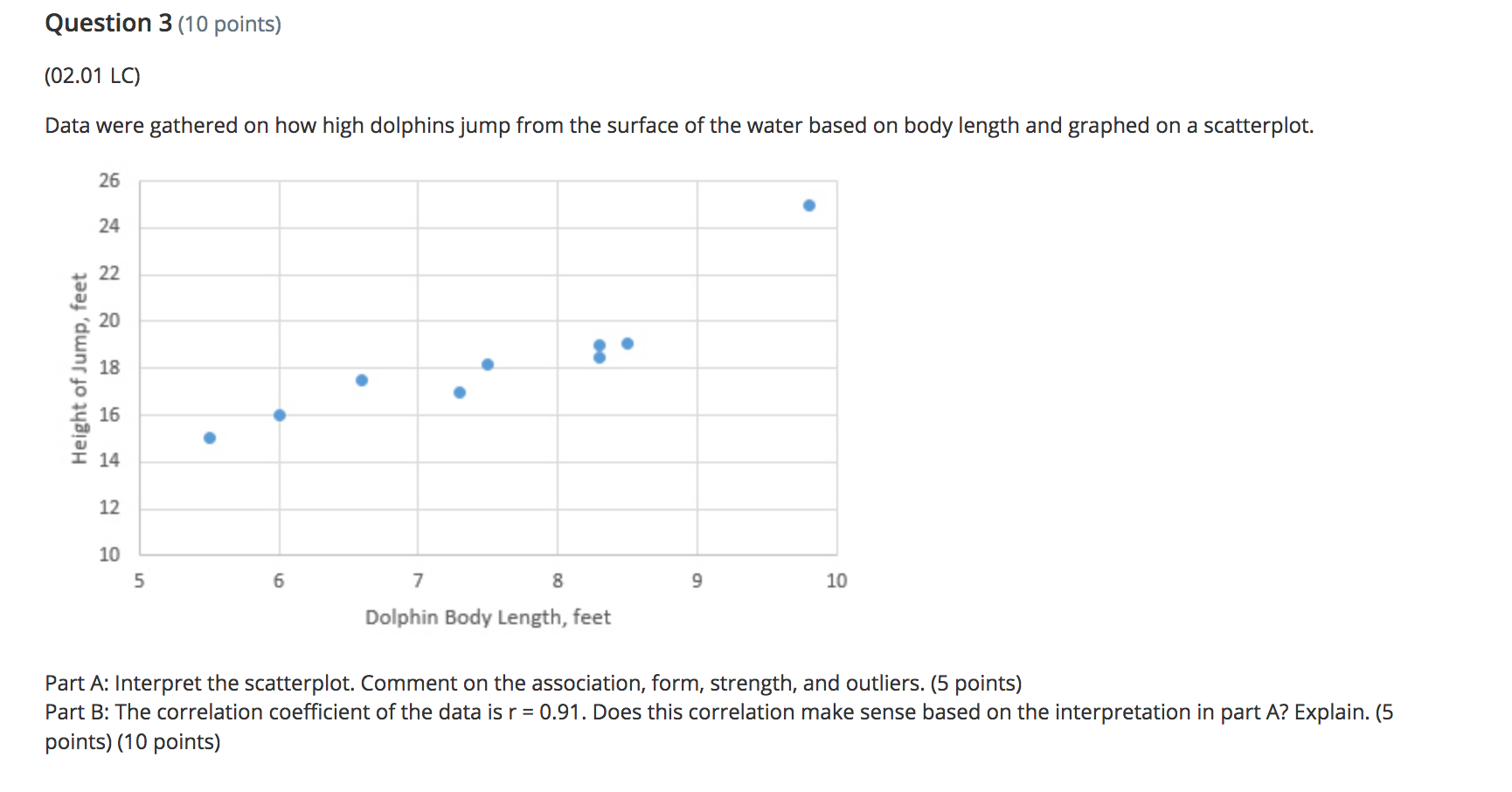
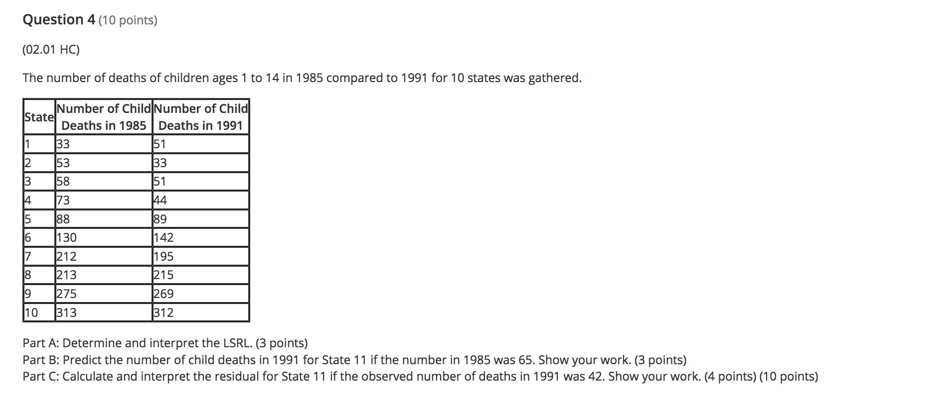
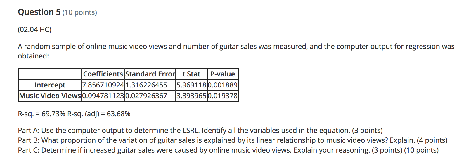
Question 2 (4 points) (02.02 MC) The regression equation for change in temperature, y, to amount of snow. 5, is given by V = 1.1 - 2.65. On Friday. the observed amount of snow was 1.3 inches and the temperature change was 1.2 degrees. Find and interpret the residual. (4 points) A a 1.08. The regression line underpredicts the temperature change. A b 1.08. The regression line overpredicts the temperature change. A: c 3.32. The regression line overpredicts the temperature change. A d -3.48. The regression line overpredicts the temperature change. e 3.48. The regression line underpredicts the temperature change. Question 3 (5 points) (02.05 MC) Two measures, x and y, were taken on 10 subjects The first of two regressions, regression 1, yielded log y = 0.027935 + 1.0026x and had the following residual plot: 0.02 0.01 2 6 8 10 . 12 14 -0.01 -0.02 -0.03 -0.04Question 4 (4 points) (02.04 LC) The computer regression output is given by Coefficients Standard Error t Stat P-value Intercept 2.218181818 1.10755 2.002783 0.07621 Year 1.054545455 0.163299 6.457746 0.000117 What are the values for a and b in the equation y = a + bx? (4 points) a a = 1.0545, b = 2.2182 Ob a = 2.2182, b = 1.0545 O c a = 1.1076, b = 0.1633 O d a = 0.1633, b = 1.1076 O e a = 2.0028, b = 6.4577Question 5 (4 points) (02.01 MC) Which scatterplot shows a strong, negative correlation with no apparent outliers? (4 points) O a 5 4.5 4 3.5 3 2.5 2 1.5 0.5 0 0 1 2 3 4 5 6 7\f\fQuestion 6 (4 points) (02.04 MC) The relationship of miles per gallon of SUVs to weight is represented by the following scatterplot: 4000 3500 3000 Weight 2500 2000 1500 1000 15 17 19 21 23 25 27 29 31 33 MPGBeatrice created the following residual plot: Residual MPG Does her residual plot make sense based on the scatterplot? Explain. (4 points) a The random residual plot makes sense because the scatterplot appears to have a negative relationship. I\" b The random residual plot does not make sense because it should have a linear relationship like the scatterplot. CI c The random residual plot does not make sense because it should have a nonlinear curve as the scatterplot is negative. K' d The random residual plot makes sense because the scatterplot appears to have a linear relationship. A e Unable to determine the residual plot because the LSRL is not given. Question 7 (4 points) (02.01 LC) Which correlation coefficient represents a strong, negative linear relationship? (4 points) Oa r = 0 Ob r = 0.21 O c r = -0.21 O d r = 0.97 O e r =-0.97Question 8 (5 points) (02.04 MC) The mean and standard deviation for male human births in the U.S. from 1995 to 2012 are i = 245,673 and 5x = 28,357. The mean and standard deviation for female human births in the US. for the same time period are \\7 = 251,785 and sy = 25,437. The correlation coefcient is r = 0.91. Find the equation for the least-squares regression line for male to female human births. (5 points) \"T,- a \\7 = 0.82 + 51,243.42x \"T b \\7 = 51,243.42 + 0.82x \"T c \\7 = 51,243.42 + 0.91x \"T d '7 = 245,673 + 0.91x \"T e \\7 = 251,785 + 0.82x Question 9 (4 points) (02.02 MC) Let fat be the explanatory variable and calories be the response variable; which scenario best describes y = 121 + 1.42x? (4 points) Oa The amount of calories in a cheeseburger increases by 1.42 for every one gram of fat. The calorie amount estimated by this model is 121 if there are zero grams of fat. Ob The amount of calories in a cheeseburger increases by 121 for every one gram of fat. The calorie amount estimated by this model is 1.42 if there are zero grams of fat. O c The amount of fat in a cheeseburger increases by 121 grams for every one calorie. The fat amount estimated by this model is 1.42 grams if there are zero calories. O d The amount of fat in a cheeseburger increases by 1.42 grams for every one calorie. The fat amount estimated by this model is 121 grams if there are zero calories. O e The amount of calories in a cheeseburger increases by 1.42 when there are zero grams of fat. The calorie amount estimated by this model is 121 if there is one gram of fat.\fQuestion 11 (4 points) (02.05 LC) Suppose that the scatterplot of log x and y shows a strong positive correlation close to 1. Which of the following is true? (4 points) A a A scatterplot of the variables x and y shows a strong nonlinear pattern. A b The variables x and y also have a correlation close to 1. A c A scatterplot of the variables log x and log y shows a strong nonlinear pattern. A- d The residual plot of the variables x and y shows a random pattern. e A residual plot of the variables log x and y shows a nonrandom pattern. Question 12 (4 points) (02.02 LC) Using the equation y = 5.4 + 1.7x, what is the predicted value if x is 1.2? (4 points) Oa 3.36 Ob -3.36 O c 7.44 Od -7.44 Oe -2.47Question 1 (10 points) (02.05 LC) Prior to fitting a linear regression model with x and y variables, the y variable was transformed by performing a cube root. The following computer output was produced. -mm man-- Rsq. = 80.34% Rsq.(adj) = 82.56% Part A: Interpret the value of r2. (5 points) Part B: Assuming the residual plot of the transformed data shows a pattern, comment on the appropriateness of this linear regression for modeling the relationship between the transformed variables. (5 points) (10 points) Question 2 (10 points) (02.04 MC) The mean unemployment rate in February of each year from 1990 to 2000 is i = 5.65, with a standard deviation of 5x = 0.92. The mean unemployment rate in July of each year for the same time frame is y = 5.62, with a standard deviation of sy = 1.3. The correlation coefcient is r = 0.91. Part A: Find the equation of the leastsquares regression line for predictingjuly unemployment rate from February's unemployment rate. Show your work. (4 points) Part B: Use the regression line to predict the unemployment rate if February's rate is 3.8. Show your work. (4 points) Part C: Find and interpret r-squared. (3 points) (10 points) Question 3 (10 points) (02.01 LC) Data were gathered on how high dolphins jump from the surface of the water based on body length and graphed on a scatterplot. 26 24 Height of Jump, feet 22 20 18 8 . 16 14 12 10 5 6 7 8 LD 10 Dolphin Body Length, feet Part A: Interpret the scatterplot. Comment on the association, form, strength, and outliers. (5 points) Part B: The correlation coefficient of the data is r = 0.91. Does this correlation make sense based on the interpretation in part A? Explain. (5 points) (10 points)Question 4 (1 0 points) (02.01 HC) The number of deaths of children ages 1 to 14 in 1985 compared to 1991 for 10 states was gathered. Number of Child Number of Child Deaths in 1985 Deaths in 1991 Part A: Determine and interpret the LSRL. (3 points) Part B: Predictthe number of child deaths in 1991 for State 11 ifthe number in 1985 was 65. Show your work. (3 points) Part C: Calculate and interpret the residual for State 11 if the observed number of deaths in 1991 was 42. Show your work. (4 points) (1 0 points) Question 5 (10 points) (02.04 HC) A random sample of online music video views and number of guitar sales was measured, and the computer output for regression was obtained: Standard Erro P-value M735671092 1316226455 .96911 .001889 Music Video Views 0.094781123 0.027926367 .39396 0.019378 Rsq. = 69.73% Rsq. (adj) = 63.68% Part A: Use the computer output to determine the LSRL. Identify all the variables used in the equation. (3 points) Part B: What proportion of the variation of guitar sales is explained by its linear relationship to music video views? Explain. (4 points) Part C: Determine if increased guitar sales were caused by online music video views. Explain your reasoning. (3 points) (10 points)