Question:

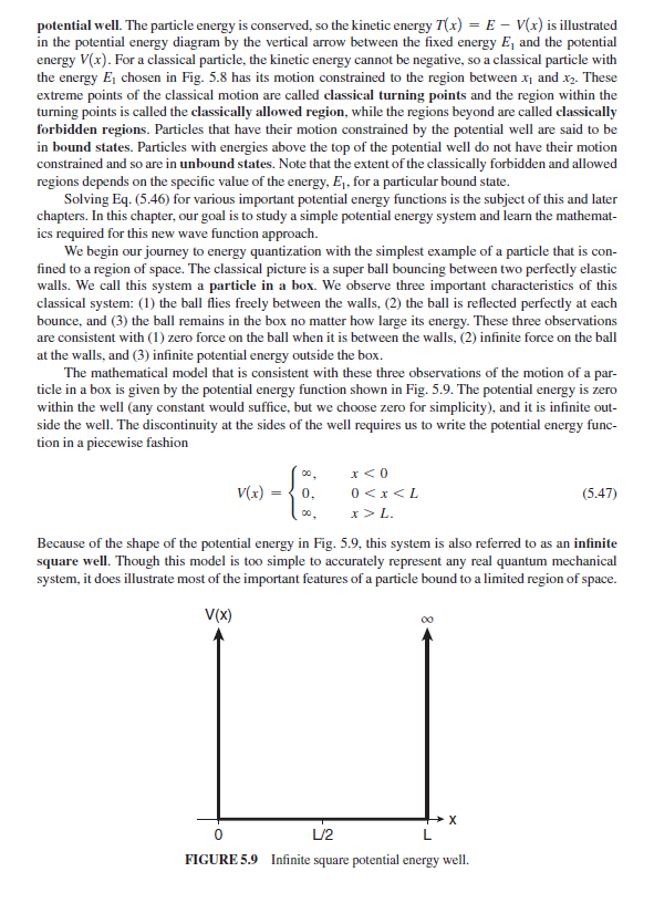
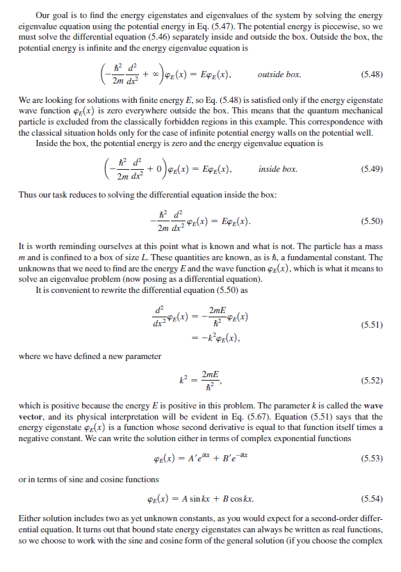
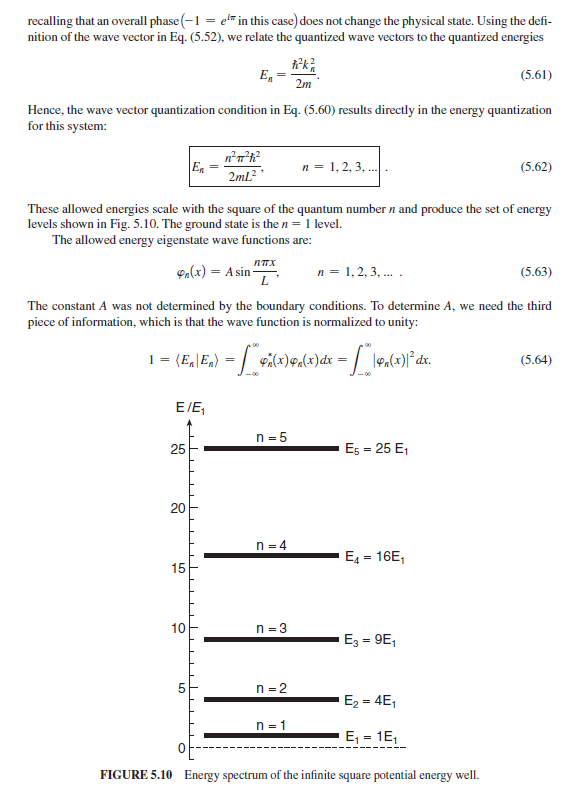
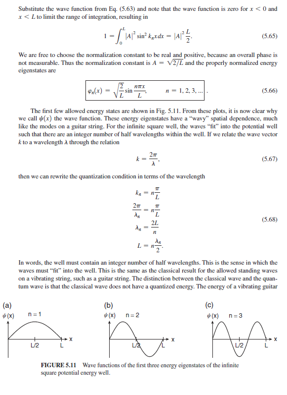
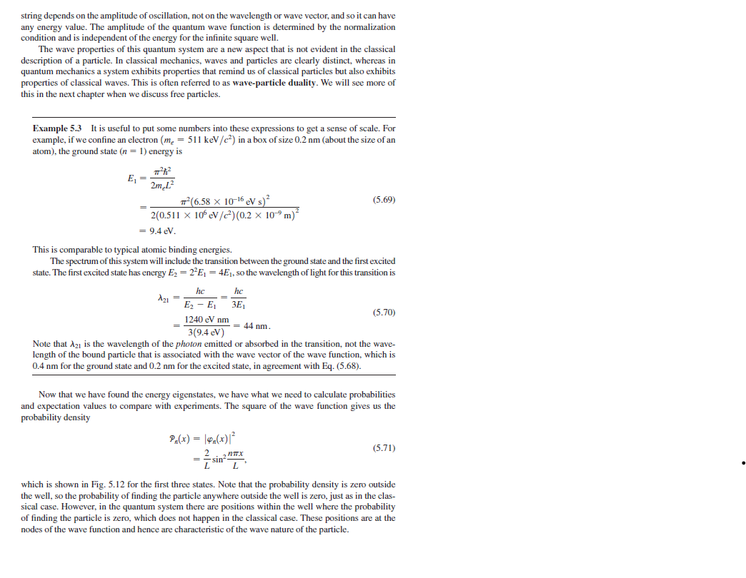
2. Consider a particle in an infinite square well. It is in the initial state y(x, 0) = A [$1(x) + $2(x)] where on (x) is the energy eigenfunctions for the infinite square well. (a) Plot (x, 0) and ly (x, 0) |2. (b) Find the wave function (x, t) at a later time t. (c) Calculate (x(t)). (d) Calculate (p(t)) and show that in this case d(x) (p) = m dt (This is true in general and is part of Ehrenfest's theorem). (e) Suppose you measure the energy of the particle at time t. What are the possible results, and what are the probabilities of getting each result?Our task now is to solve the energy eigenvalue equation, which we found to be a differential equation 2 m dez + V (x) FF (x) = EFF(x). (5.46) As you might expect, the solutions to this differential equation depend critically on the functional dependence of the potential energy V(x). A generic potential energy function is depicted in Fig. 5.8 in a potential energy diagram that illustrates some important aspects of the motion of the particle. Most of the interesting systems to which we will apply Eq. (5.46) resemble the potential energy func- tion depicted in Fig. 5.8 in that V(x) has a minimum, so we refer to the potential energy function as a Energy Classically Classically allowed region - - Classically forbidden region forbidden region Classical turning points T = E-V(x) V(x) - X X1 X2 FIGURE 5.8 A generic potential energy well.potential well. The particle energy is conserved, so the kinetic energy (x) = E - V(x) is illustrated in the potential energy diagram by the vertical arrow between the fixed energy E, and the potential energy V(x). For a classical particle, the kinetic energy cannot be negative, so a classical particle with the energy E, chosen in Fig. 5.8 has its motion constrained to the region between x and x2. These extreme points of the classical motion are called classical turning points and the region within the turning points is called the classically allowed region, while the regions beyond are called classically forbidden regions. Particles that have their motion constrained by the potential well are said to be in bound states. Particles with energies above the top of the potential well do not have their motion constrained and so are in unbound states. Note that the extent of the classically forbidden and allowed regions depends on the specific value of the energy, E, for a particular bound state. Solving Eq. (5.46) for various important potential energy functions is the subject of this and later chapters. In this chapter, our goal is to study a simple potential energy system and learn the mathemat- ics required for this new wave function approach. We begin our journey to energy quantization with the simplest example of a particle that is con- fined to a region of space. The classical picture is a super ball bouncing between two perfectly elastic walls. We call this system a particle in a box. We observe three important characteristics of this classical system: (1) the ball flies freely between the walls, (2) the ball is reflected perfectly at each bounce, and (3) the ball remains in the box no matter how large its energy. These three observations are consistent with (1) zero force on the ball when it is between the walls, (2) infinite force on the ball at the walls, and (3) infinite potential energy outside the box. The mathematical model that is consistent with these three observations of the motion of a par- ticle in a box is given by the potential energy function shown in Fig. 5.9. The potential energy is zero within the well (any constant would suffice, but we choose zero for simplicity), and it is infinite out- side the well. The discontinuity at the sides of the well requires us to write the potential energy func- tion in a piecewise fashion V(x) 0 L. Because of the shape of the potential energy in Fig. 5.9, this system is also referred to as an infinite square well. Though this model is too simple to accurately represent any real quantum mechanical system, it does illustrate most of the important features of a particle bound to a limited region of space. V(x) 00 X 0 L/2 FIGURE 5.9 Infinite square potential energy well.Our goal is to find the energy eigenstates and eigenvalues of the system by solving the energy eigenvalue equation using the potential energy in Eq. (5.47). The potential energy is piecewise, so we must solve the differential equation (5.46) separately inside and outside the box. Outside the box, the potential energy is infinite and the energy eigenvalue equation is 2m diz + 0 PE ( x ) = EVE( x ) , outside box. (5.48) We are looking for solutions with finite energy E, so Eq. (5.48) is satisfied only if the energy eigenstate wave function 4 (x) is zero everywhere outside the box. This means that the quantum mechanical particle is excluded from the classically forbidden regions in this example. This correspondence with the classical situation holds only for the case of infinite potential energy walls on the potential well. Inside the box, the potential energy is zero and the energy eigenvalue equation is 2 m de + 0 ) 9 :(x) = EFE(x ) , inside box. (5.49) Thus our task reduces to solving the differential equation inside the box: h2 d2 2m dx? PE (X) = EQE(x). (5.50) It is worth reminding ourselves at this point what is known and what is not. The particle has a mass m and is confined to a box of size L. These quantities are known, as is h, a fundamental constant. The unknowns that we need to find are the energy E and the wave function or(x), which is what it means to solve an eigenvalue problem (now posing as a differential equation). It is convenient to rewrite the differential equation (5.50) as d2 2mE dx 240 E (x ) = - 12 PE(x) (5.51) = -KE(x). where we have defined a new parameter A2 - 2mE 1: 2 (5.52) which is positive because the energy E is positive in this problem. The parameter & is called the wave vector, and its physical interpretation will be evident in Eq. (5.67). Equation (5.51) says that the energy eigenstate o (x) is a function whose second derivative is equal to that function itself times a negative constant. We can write the solution either in terms of complex exponential functions PE(x) = A'e + B'e-x (5.53) or in terms of sine and cosine functions PE(x) = A sinkx + B coskx. (5.54) Either solution includes two as yet unknown constants, as you would expect for a second-order differ- ential equation. It turns out that bound state energy eigenstates can always be written as real functions, so we choose to work with the sine and cosine form of the general solution (if you choose the complexexponential form, you will arrive at the sine and cosine solutions at the end of the problem anyway: Problem 5.3). Hence the energy eigenstate wave function throughout space is PE(x) = L. We now need some more information to reach the final solution. There are three unknowns in the problem: A, B, and & [ which contains the energy E through Eq. (5.52)], so we expect to need three pieces of information to solve for the three unknowns. We get two of these pieces of information from imposing boundary conditions on the wave function. To make sure that the mathematical solutions properly represent real physical systems, we require that the wave function be continuous across each boundary between different regions of space where different solutions exist. Applying this require- ment on the continuity of the wave function at the sides of the box x = 0 and L yields two boundary condition equations: (0): Asin(0) + Bcos(0) = 0 (5.56) PE(L): A sinkl + BcoskL = 0. The boundary condition at the left side of the box yields B = 0. (5.57) This tells us that the cosine part of the general solution is not allowed because the cosine solution is not zero at the edge of the box and so does not match the wave function outside the box. The exclusion of the cosine part of the solution arises because we chose to locate our box with one side at x = 0; if the box is located differently, then both sine and cosine solutions may be allowed. Given that the allowed wave functions must be sine functions, the boundary condition at the right side of the box yields A sinkl = 0. (5.58) This equation is satisfied if A = 0, but that yields a wave function that is zero everywhere, so it is unin- teresting. The more interesting possibility is that sinkL = 0. (5.59) This is a transcendental equation that places limitations on the allowed values of the wave vector k. We will find other transcendental equations when we study other potentials. This transcendental equation has solutions when the sinusoid function is zero. Hence the wave vectors that satisfy this equation are KL = AT (5.60) Kn = 1- n = 1, 2, 3, ... . Only discrete wave vectors are allowed, so this is termed the quantization condition. The index n is the quantum number, which we use to label the quantized states and energies. The value n = 0 is excluded because that would yield a wave function equal to zero, which is uninteresting. The nega- tive values of n are excluded because they yield the same states as the corresponding positive n values,recalling that an overall phase (-1 = elf in this case) does not change the physical state. Using the defi- nition of the wave vector in Eq. (5.52), we relate the quantized wave vectors to the quantized energies E, = (5.61) Hence, the wave vector quantization condition in Eq. (5.60) results directly in the energy quantization for this system: E = ! 2ml2' n = 1, 2, 3, ... (5.62) These allowed energies scale with the square of the quantum number n and produce the set of energy levels shown in Fig. 5.10. The ground state is the n = 1 level. The allowed energy eigenstate wave functions are: On(x) = Asin- L n = 1, 2. 3. ... . (5.63) The constant A was not determined by the boundary conditions. To determine A, we need the third piece of information, which is that the wave function is normalized to unity: 1 = (E, | E. ) = / 4:(x)en (x)dx - / 14.(x)12 ax. (5.64) E/E n = 5 25 TTTT Es = 25 E1 20 n =4 EA = 1651 15 TTTTTT | TTTT TTTT 10 n = 3 Eg = 961 5 n = 2 E2 = 461 n =1 E1 = 16 FIGURE 5.10 Energy spectrum of the infinite square potential energy well.Substitute the wave function from Eq. (5.63) and note that the wave function is zero for x