question 5.3 and the table is attached in the second picture

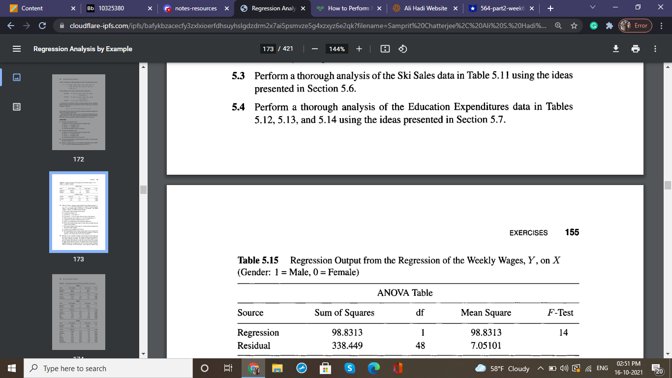
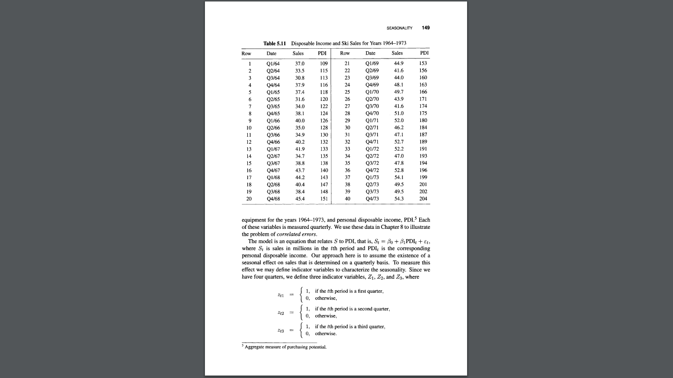
Content X Bb 10325380 X notes-resources x 5 Regression Analy X olo How to Perform | X Ali Hadi Website X *564-part2-week6 x + X C cloudflare-ipfs.com/ipfs/bafykbzacecfy3zxlxioerfdhsuyhslgdzdrms7ai5psmvze5g4xzxyz6e2qk?filename=Samprit%20Chatterjee%20%20Ali%20S.%20Hadi%.. G Error Regression Analysis by Example 173 / 421 144% + 5.3 Perform a thorough analysis of the Ski Sales data in Table 5.11 using the ideas presented in Section 5.6. 5.4 Perform a thorough analysis of the Education Expenditures data in Tables 5.12, 5.13, and 5.14 using the ideas presented in Section 5.7. 172 EXERCISES 155 173 Table 5.15 Regression Output from the Regression of the Weekly Wages, Y, on X (Gender: 1 = Male, 0 = Female) ANOVA Table Source Sum of Squares df Mean Square F-Test Regression 98.8313 1 98.8313 14 Residual 338.449 48 7.05101 Type here to search O S 02:51 PM 58'F Cloudy ~ D() ENG 16-10-2021 20SEASONALITY 149 Table 5.11 Disposable Income and Ski Sales for Years 1964-1973 Row Dat Sales PD Row Date Sales PDI 01/64 37.0 109 21 01/69 44.9 153 02/64 33.5 115 22 Q2/69 41.6 156 Q3/64 30.8 113 23 Q3/69 44.0 160 04/64 $7.9 116 24 04/69 48.1 163 HOWAWN Q1/65 37.4 118 25 21/70 19.7 166 Q2/65 31.6 120 26 02/70 43 9 171 03/65 34.0 122 27 Q3/70 41.6 174 Q4/65 38.1 124 28 Q4/70 51.0 175 Q1/6 10.0 126 29 Q1/71 52.0 180 Q2/6 35.0 128 30 Q2/71 46.2 184 Q3/66 34.9 130 31 Q3/71 47.1 187 Q4/66 40.2 132 32 04/71 52.7 189 Q1/67 1.9 133 Q1/72 52.2 191 Q2/6 347 135 34 Q2/72 17.0 193 Q3/67 38.8 138 35 Q3/72 47.8 194 Q4/67 13.7 140 36 Q4/72 52.8 196 17 Q1/68 14.2 143 37 01/73 54 1 199 18 Q2/68 40.4 147 38 Q2/73 19.5 201 19 Q3/68 38.4 148 39 Q3/73 19 5 202 20 Q4/68 45.4 151 40 04/73 54.3 204 equipment for the years 1964-1973, and personal disposable income, PDI. Each of these variables is measured quarterly. We use these data in Chapter 8 to illustrate the problem of correlated errors. The model is an equation that relates S to PDI, that is, St = Po + 8PDI, + Et, where S, is sales in millions in the tth period and PDI, is the corresponding personal disposable income. Our approach here is to assume the existence of a seasonal effect on sales that is determined on a quarterly basis. To measure this effect we may define indicator variables to characterize the seasonality. Since we have four quarters, we define three indicator variables, 21, Z2, and Za, where 21 = 1, if the tth period is a first quarter, otherwise, . if the tth period is a second quarter, 0, otherwise, = 1, if the tth period is a third quarter, 0 , otherwise Aggregate measure of purchasing potential