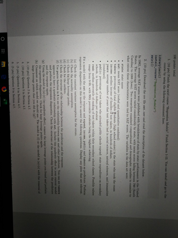
Question2. I really don't know how to code it.

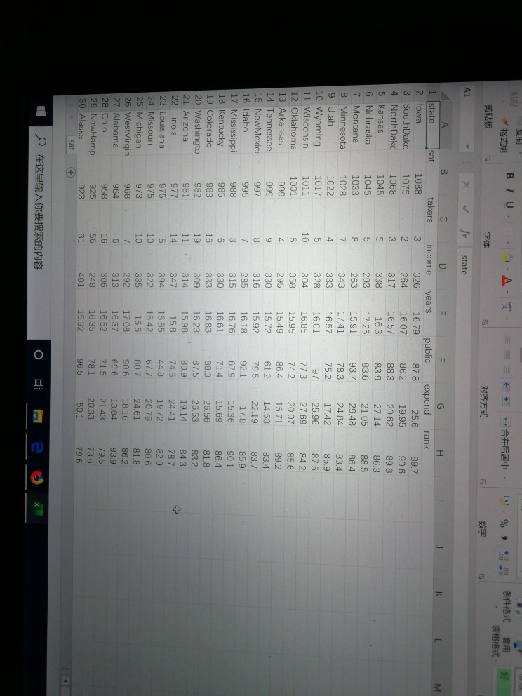
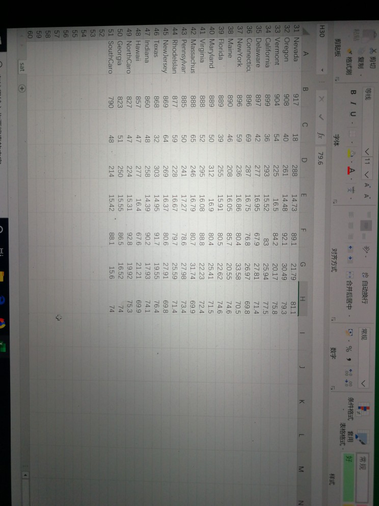
100 points total 1. (10 pts) Finish the swirl course "Regression Models". Finish Section 1-13. You can install and go to the course by using the following command lines. library(swirl) install_course ("Regression_Models") swirl 2. (10 pts) Download the esv file sat.csv and read the description of the dataset below. In 1982, average SAT scores were published with breakdowns of state-by-state performance in the United States. The average SAT scores varied considerably by state, with mean scores falling between 790 (South Carolina) to 1088 (Iowa). Two researchers examined compositional and demographie variables to examine to what extent these characteristics were tied to SAT scores. The variables in the data set were: state: state name sat: mean SAT score (verbal and quantitative combined) takers: percentage of total eligible ftudents (high school seniors) in the state who took the exam income: median income of families of test takers, in hundreds of dollars. years: average number of years that test takers had in social sciences, natural sciences, and humanities (combined) public: percentage of test takers who attended public schools expend: state expenditure on secondary schools, in hundreds of dollars per student rank: median percentile of ranking of test takers within their secondary school classes. Possible values range from 0-99, with 99th percentile students being the highest achieving. Fit a model with the sat as the response and expend, income, public and takers as predictors. Perform regression diagnostics on this model to answer the following questions. Display any plots that are relevent. (a) Check the constant variance assumption for the errors. (b) Check the normality assumption. (c) Check for large leverage points. (d) Check for the outliers. (e) Check the structure of the relationship between the predictors and the response. (I) Use pairs function in R to see the relationship between sat and other predictors. You can see takers appears to have a quadratic relationship with sat. Include this quadratic effect in your current model and perform the regression diagnostics. Check the structure of the relationship between the predictors and the response again. (g) Using the model in (a)-(e) (no quadratic effect), remove the large leverage points you found and perform the regression diagnostics. Check for large leverage points agnin (h) Comment on which model we should use. The model in (I) or the model in (a)-(e) with the removal of large leverage points that you did in (s)? 3. (10 pts) Question 2 in Section 4.7. 4. (10 pts) Question 5 in Section 4.7. 5. (5 pts) Question 6 in Section 4.7. 6. (5 pts) Question 9 in Section 4.7. 17 &1818 A1 K L M 12CFI BUA A#684. 0. % BENDE ** 5 X fx state A B C D E F G III 1 state sat takers income years public expend rank 2 lowa 1088 326 16.79 87.8 25.6 89.7 3 South Dako 1075 264 16.07 86.2 19.95 90.6 4 North Dako 1068 317 16.57 88.3 20.62 89.8 5 Kansas 1045 338 16.3 83.9 27.14 86.3 6 Nebraska 1045 293 17.25 83.6 21.05 88.5 7 Montana 1033 263 15.91 93.7 29.48 86.4 8 Minnesota 1028 343 17.41 78,3 24.84 83.4 9 Utah 1022 333 16.57 75.2 17.42 85.9 10 Wyoming 1017 328 16.01 97 25.96 87.5 11 Wisconsin 1011 304 16.85 77.3 27.69 84.2 12 Oklahoma 1001 358 15.95 74.2 20.07 85.6 13 Arkansas 999 295 15.49 86.4 15.71 89.2 14 Tennessee 999 330 15.72 61.2 14.58 83.4 15 New Mexico 997 316 15.92 79.5 22.19 83.7 16 Idaho 995 285 16.18 921 17.8 85.9 17 Mississippi 988 315 16.76 67.9 15.36 90.1 18 Kentucky 985 330 16.61 71.4 15.69 86.4 19 Colorado 983 333 16.83 88.3 26.56 81.8 20 Washingto 982 309 16.23 87.5 26.53 83.2 21 Arizona 981 314 15.98 80.9 19.14 84.3 22 Illinois 977 347 15.8 74.6 24.41 78.7 23 Louisiana 975 394 16.85 44.8 19.72 82.9 24 Missouri 975 322 16.42 67.7 20.79 80.6 25 Michigan 973 335 - 16.5 80.7 24.61 81.8 26 West Virgin 968 292 17.08 90.6 18.16 86.2 27 Alabama 964 313 16.37 69.6 13.84 83.9 28 Ohio 958 306 16.52 71.5 21.43 79.5 29 New Hamp 925 248 16.35 78.1 20.33 73.6 30 Alaska 923 401 15.32 96.5 50.1 79.6 sat + DOGO ABOUT I WNW EX TAPE 2 st . = 11 VA A .A. 18 # FR 2 ani A# te! BIU. . . 0. % * * Ist *** H30 X for 79.6 B C D I J K L M N 18 40 288 261 225 293 277 287 236 208 A 31 Nevada 32 Oregon 33 Vermont 34 California 35 Delaware 36 Connecticu 37 NewYork 38 Maine 39 Florida 40 Maryland 41 Virginia 42 Massachus 43 Pennsylvar 44 Rhodelslan 45 NewJersey 46 Texas 47 Indiana 48 Hawaii 49 North Caro 50 Georgia 51 South Caro 917 908 904 899 897 896 896 890 889 889 888 888 885 877 869 868 860 857 827 823 790 255 312 295 246 241 228 269 303 258 277 224 250 214 E 14.73 14.48 16.5 15.52 16.95 16.75 16.86 16.05 15.91 16.9 16.08 16.79 17.27 16.67 16.37 14.95 14.39 16.4 15.31 15.55 15.42 F 89.1 92.1 84.2 83 67.9 76.8 80.4 85.7 80.5 80.4 88.8 80.7 78.6 79.7 80.6 91.7 90.2 67.6 92.8 86.5 88.1 G 21.79 30.49 20.17 25.94 27.81 26.97 33.58 20.55 22.62 25.41 22.23 31.74 27.98 25.59 27.91 19.55 17.93 21.21 19.92 16.52 15.6 H 81.1 79.3 75.8 77.5 71.4 69.8 70.5 74.6 74.6 71.5 72.4 69.9 73.4 71.4 69.8 76.4 74.1 69.9 75.3 74 74 sat + 100 points total 1. (10 pts) Finish the swirl course "Regression Models". Finish Section 1-13. You can install and go to the course by using the following command lines. library(swirl) install_course ("Regression_Models") swirl 2. (10 pts) Download the esv file sat.csv and read the description of the dataset below. In 1982, average SAT scores were published with breakdowns of state-by-state performance in the United States. The average SAT scores varied considerably by state, with mean scores falling between 790 (South Carolina) to 1088 (Iowa). Two researchers examined compositional and demographie variables to examine to what extent these characteristics were tied to SAT scores. The variables in the data set were: state: state name sat: mean SAT score (verbal and quantitative combined) takers: percentage of total eligible ftudents (high school seniors) in the state who took the exam income: median income of families of test takers, in hundreds of dollars. years: average number of years that test takers had in social sciences, natural sciences, and humanities (combined) public: percentage of test takers who attended public schools expend: state expenditure on secondary schools, in hundreds of dollars per student rank: median percentile of ranking of test takers within their secondary school classes. Possible values range from 0-99, with 99th percentile students being the highest achieving. Fit a model with the sat as the response and expend, income, public and takers as predictors. Perform regression diagnostics on this model to answer the following questions. Display any plots that are relevent. (a) Check the constant variance assumption for the errors. (b) Check the normality assumption. (c) Check for large leverage points. (d) Check for the outliers. (e) Check the structure of the relationship between the predictors and the response. (I) Use pairs function in R to see the relationship between sat and other predictors. You can see takers appears to have a quadratic relationship with sat. Include this quadratic effect in your current model and perform the regression diagnostics. Check the structure of the relationship between the predictors and the response again. (g) Using the model in (a)-(e) (no quadratic effect), remove the large leverage points you found and perform the regression diagnostics. Check for large leverage points agnin (h) Comment on which model we should use. The model in (I) or the model in (a)-(e) with the removal of large leverage points that you did in (s)? 3. (10 pts) Question 2 in Section 4.7. 4. (10 pts) Question 5 in Section 4.7. 5. (5 pts) Question 6 in Section 4.7. 6. (5 pts) Question 9 in Section 4.7. 17 &1818 A1 K L M 12CFI BUA A#684. 0. % BENDE ** 5 X fx state A B C D E F G III 1 state sat takers income years public expend rank 2 lowa 1088 326 16.79 87.8 25.6 89.7 3 South Dako 1075 264 16.07 86.2 19.95 90.6 4 North Dako 1068 317 16.57 88.3 20.62 89.8 5 Kansas 1045 338 16.3 83.9 27.14 86.3 6 Nebraska 1045 293 17.25 83.6 21.05 88.5 7 Montana 1033 263 15.91 93.7 29.48 86.4 8 Minnesota 1028 343 17.41 78,3 24.84 83.4 9 Utah 1022 333 16.57 75.2 17.42 85.9 10 Wyoming 1017 328 16.01 97 25.96 87.5 11 Wisconsin 1011 304 16.85 77.3 27.69 84.2 12 Oklahoma 1001 358 15.95 74.2 20.07 85.6 13 Arkansas 999 295 15.49 86.4 15.71 89.2 14 Tennessee 999 330 15.72 61.2 14.58 83.4 15 New Mexico 997 316 15.92 79.5 22.19 83.7 16 Idaho 995 285 16.18 921 17.8 85.9 17 Mississippi 988 315 16.76 67.9 15.36 90.1 18 Kentucky 985 330 16.61 71.4 15.69 86.4 19 Colorado 983 333 16.83 88.3 26.56 81.8 20 Washingto 982 309 16.23 87.5 26.53 83.2 21 Arizona 981 314 15.98 80.9 19.14 84.3 22 Illinois 977 347 15.8 74.6 24.41 78.7 23 Louisiana 975 394 16.85 44.8 19.72 82.9 24 Missouri 975 322 16.42 67.7 20.79 80.6 25 Michigan 973 335 - 16.5 80.7 24.61 81.8 26 West Virgin 968 292 17.08 90.6 18.16 86.2 27 Alabama 964 313 16.37 69.6 13.84 83.9 28 Ohio 958 306 16.52 71.5 21.43 79.5 29 New Hamp 925 248 16.35 78.1 20.33 73.6 30 Alaska 923 401 15.32 96.5 50.1 79.6 sat + DOGO ABOUT I WNW EX TAPE 2 st . = 11 VA A .A. 18 # FR 2 ani A# te! BIU. . . 0. % * * Ist *** H30 X for 79.6 B C D I J K L M N 18 40 288 261 225 293 277 287 236 208 A 31 Nevada 32 Oregon 33 Vermont 34 California 35 Delaware 36 Connecticu 37 NewYork 38 Maine 39 Florida 40 Maryland 41 Virginia 42 Massachus 43 Pennsylvar 44 Rhodelslan 45 NewJersey 46 Texas 47 Indiana 48 Hawaii 49 North Caro 50 Georgia 51 South Caro 917 908 904 899 897 896 896 890 889 889 888 888 885 877 869 868 860 857 827 823 790 255 312 295 246 241 228 269 303 258 277 224 250 214 E 14.73 14.48 16.5 15.52 16.95 16.75 16.86 16.05 15.91 16.9 16.08 16.79 17.27 16.67 16.37 14.95 14.39 16.4 15.31 15.55 15.42 F 89.1 92.1 84.2 83 67.9 76.8 80.4 85.7 80.5 80.4 88.8 80.7 78.6 79.7 80.6 91.7 90.2 67.6 92.8 86.5 88.1 G 21.79 30.49 20.17 25.94 27.81 26.97 33.58 20.55 22.62 25.41 22.23 31.74 27.98 25.59 27.91 19.55 17.93 21.21 19.92 16.52 15.6 H 81.1 79.3 75.8 77.5 71.4 69.8 70.5 74.6 74.6 71.5 72.4 69.9 73.4 71.4 69.8 76.4 74.1 69.9 75.3 74 74 sat +