

Questions are in 1.1 and 1.2 png, and the data is in the Table+number.png
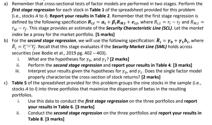
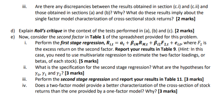
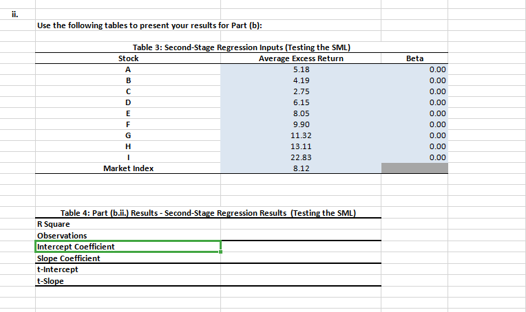
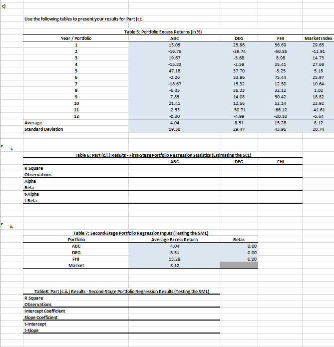
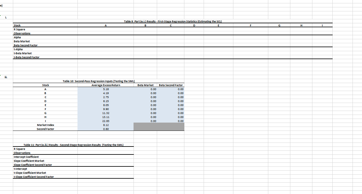
a] Remember that cross-sectional tests of factor models are performed in two stages. Perform the rst stage regression for each stock in Tobie 1 of the spreadsheet provided for this problem [i.e., stocks A to 1]. Report your results in Table 2. Remember that the first stage regression is dened by the following specification \"at = a. + n,\" + em, where Ru = r]- r, and R,\" = r\" i}; This stage provides an estimate of the Security inmdestic Line [SCI]. Let the market index be a proxy for the market portfolio. [5 marks] b} For the secoml stage repression. we will use the following specification: it, = yo + hill. where f7; = W. Recall that this stage evaluates if the Securfty Market Una [Sou] holds across securities {see Bodie et al.. 2mg pg. 402 403]. i. What are the hypotheses for ya, and y]? [2 marks] ii. Perform the second stage repression and report your results in Table l. [3 marks] ili. Interpret 1[tour results given the hypotheses for ya. and n. Does the single factor mode! properlyr characterize the cross-section of stock returns? [2 marks] c] Table 5 of the spreadsheet provided for this problem groups the nine stocks in the sample {I.e.. stocksA to i] into three portfolios that maximize the dispersion of betas In the resulting portfolios. i. Use this data to conduct the 'rststnge repression on the three portfolios and report your results in Table 6. [3 marks] Ii. Conduct the second stone repression on the three portfolios and report your results In Table 8. [3 marks] III. Are there any discrepancies between the results obtained In section lcii} and toil} and those obtained In sections [a] and {b}? Why? what do these results imply about the single factor model characterization of cross-sectional stock returns? [2 marks] d} Explain Raff's critique In the context of the tests performed in (at, {hi and {c}. [2 marks] e] Now, consider the second factor in Table 1 of the spreadsheet provided for this problem. I. Perform the rst stone repression. RM = at + mm + u?\" + e\Table 1: Stock Excess Returns (in %) Year Market Index Second Factor* A B C D E F G H 1 29.65 -9.84 33.88 25.2 36.48 42.89 39.89 39.67 74.57 40.22 90.19 -11.91 6.46 -49.87 24.7 -25.11 -54.39 44.92 -54.33 -79.76 W N -71.58 -26.64 14.73 16.12 65.14 -25.04 18.91 -39.86 -3.91 -5.69 26.73 14.49 18.14 27.68 -16.51 14.46 -38.64 -23.31 -0.72 -3.21 92.39 -3.82 13.74 0.09 5.18 17.82 15.67 61.93 63.95 -32.82 44.26 -42.96 101.67 24.24 8.98 6 25.97 -13.31 -32.17 44.94 -19.56 69.42 90.43 76.72 1.72 77.22 72.38 10.64 -3.52 31.55 -74.65 50.18 74.52 15.38 21.95 -43.95 -13.4 28.95 8 1.02 8.43 -23.79 47.02 -42.28 28.61 -17.64 28.83 98.01 28.12 39.41 9 18.82 8.23 -4.59 28.69 -0.54 2.32 42.36 18.93 -2.45 37.65 94.67 10 23.92 7.06 -8.03 48.61 23.65 26.26 -3.65 23.31 15.36 80.59 52.51 11 -41.61 -15.74 78.22 -85.02 -0.79 -68.7 85.71 -45.64 2.27 -72.47 -80.26 12 -6.64 2.03 4.75 42.95 -48.6 26.27 13.24 -34.34 -54.47 -1.5 -24.46 *Used for part (e) only\fii. Use the following tables to present your results for Part (b): Table 3: Second-Stage Regression Inputs (Testing the SML) Stock Average Excess Return Beta A 5.18 0.00 B 4.19 0.00 C 2.75 0.00 D 6.15 0.00 E 8.05 0.00 9.90 0.00 G 11.32 0.00 H 13.11 0.00 22.83 0.00 Market Index 8.12 Table 4: Part (b.ii.) Results - Second-Stage Regression Results (Testing the SML) R Square Observations Intercept Coefficient Slope Coefficient t-Intercept t-SlopeUse the following tables to present your results for Part (c): Table 5: Portfolio Excess Returns [in *6) Year / Portfolio ABC DEG FHI Market Index 15.05 25.BE 56.59 29.65 -16.75 -29.74 -50.85 -11.91 19.57 -5.68 14.73 -15.63 -2.56 35.41 27.68 47.18 37.70 -3.25 5.18 6 -2.26 53.85 75.44 25.97 7 -16.57 15.32 12.50 10.64 -5.35 36.33 32.12 1.02 7.85 14.06 50.42 16.62 10 21.4 12.6 52.14 23.92 11 -2.53 -50.71 -65.12 -41.51 12 -0.30 -4.95 -20.10 5.54 Average 4.04 5.51 15.25 B.12 Standard Deviation 19.30 29.47 43.96 20.74 i. Table 6: Part (c.i.) Results - First-Stage Portfolio Regression Statistics (Estimating the 5CL) ABC DEG FHI R Square Observations Alpha Beta t-Alpha t-Beta ii. Table 7: Second-Stage Portfolio Regression Inputs (Testing the SML] Portfolio Average Excess Return Betas ABC 4.04 0.00 DEG 8.51 0.00 FHI 15.28 0.00 Market B.12 Tables: Part (Gil.) Results - Second-Stage Portfolio Regression Results (Testing the SML] R Square Observations Intercept Coefficient Slope Coefficient t-Intercept t-SlopeTable 9: Part (e.i.) Results - First-Stage Regression Statistics (Estimating the 5CL) Stock A B D E F G H R Square observations Alph Beta Market Beta Second Factor t-Alpha t-Beta Market t-Beta Second Factor iii Table 10: Second-Pass Regression Inputs (Testing the SML] Stock Average Excess Return Beta Market Beta Second Factor A 5.16 0.00 0.00 4.19 0.00 0.00 2.75 0.00 0.00 5.15 0.00 0.00 B.05 0.00 0.00 9.90 0.00 0.00 11.32 0.00 0.00 13.11 0.00 0.00 22.63 0.00 0.00 Market Index B.12 Second Factor 0.50 Table 11: Part (e. iii.] Results - Second-Stage Regression Results (Testing the SML) R Square Observations Intercept Coefficient Slope Coefficient Market Slope Coefficient Second Factor -Intercept -Slope Coefficient Market t-Slope Coefficient Second Factor
