Read Chapter 6 of the book "How to measure anything". Now, write a letter to Mr. Williams, starting with the following statement:

"Mr. Williams, currently you work with categorical risk metrics (high, medium, low). Based on a literature review, I would suggest you to consider the idea of adopting a quantitative approach based on Monte Carlo Simulations."

In the body of your letter address the following topics:

what is the issue of treating the risk as high, medium, and low; what other alternatives you know (based on the review of Chapter 6); what is the essence of the Monte Carlo method and why you would recommend its implementation; illustrate the application of Monte Carlo with an R simulation (in the letter report major results via graphs and tables accompanied by explanations and interpretation): for simplicity purposes assume a portfolio of 3 assets only; assume a weights for each asset (weights should sum up to 1); assume a lower and an upper bound on the expected returns; assume the returns of all three assets follow normal distribution; show how the risk of the portfolio might be measured via Monte Carlo simulations if all assumptions hold true.

Upload the letter and the R script.

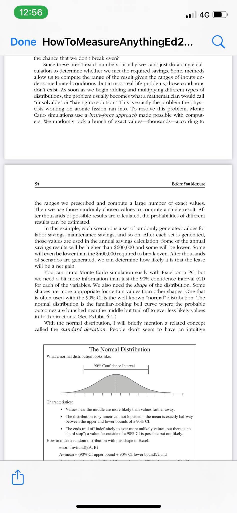
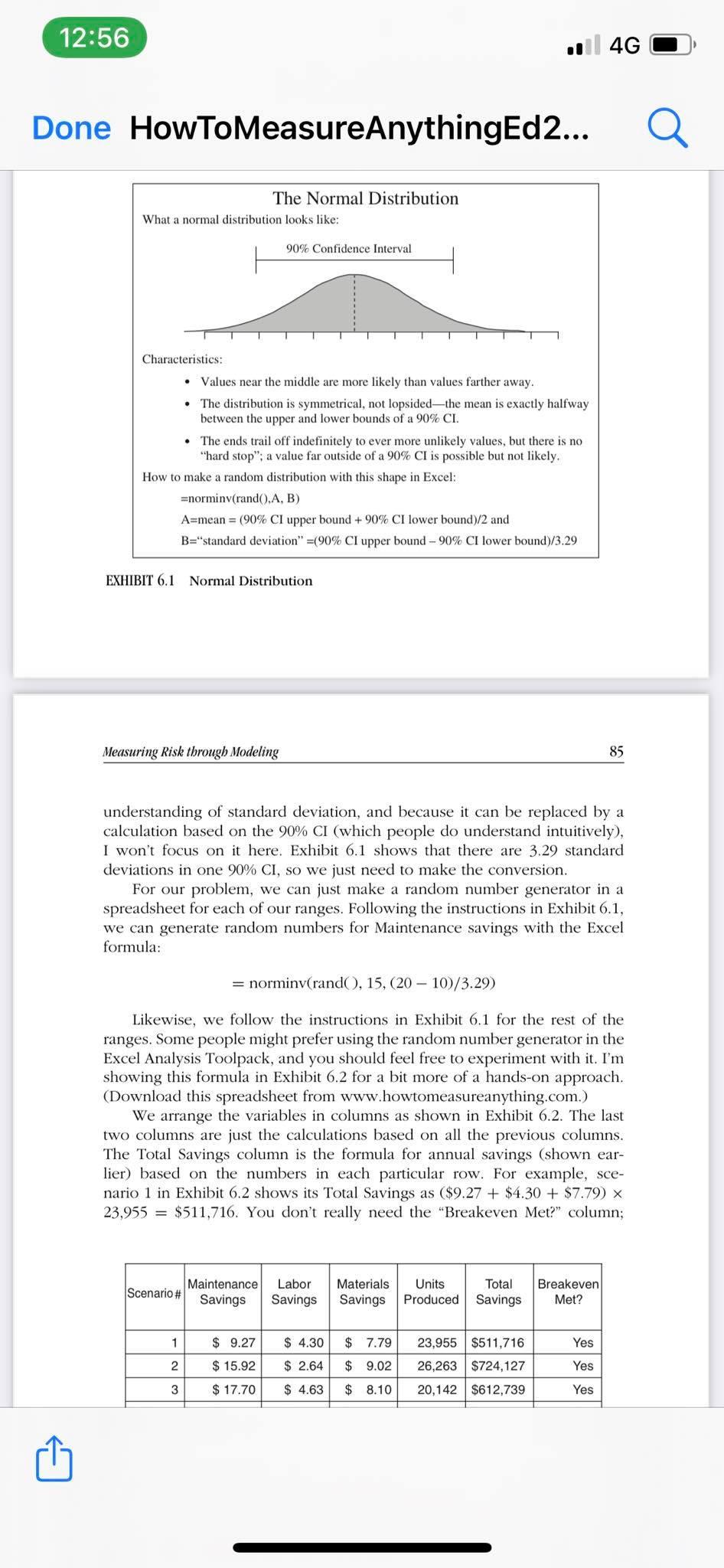
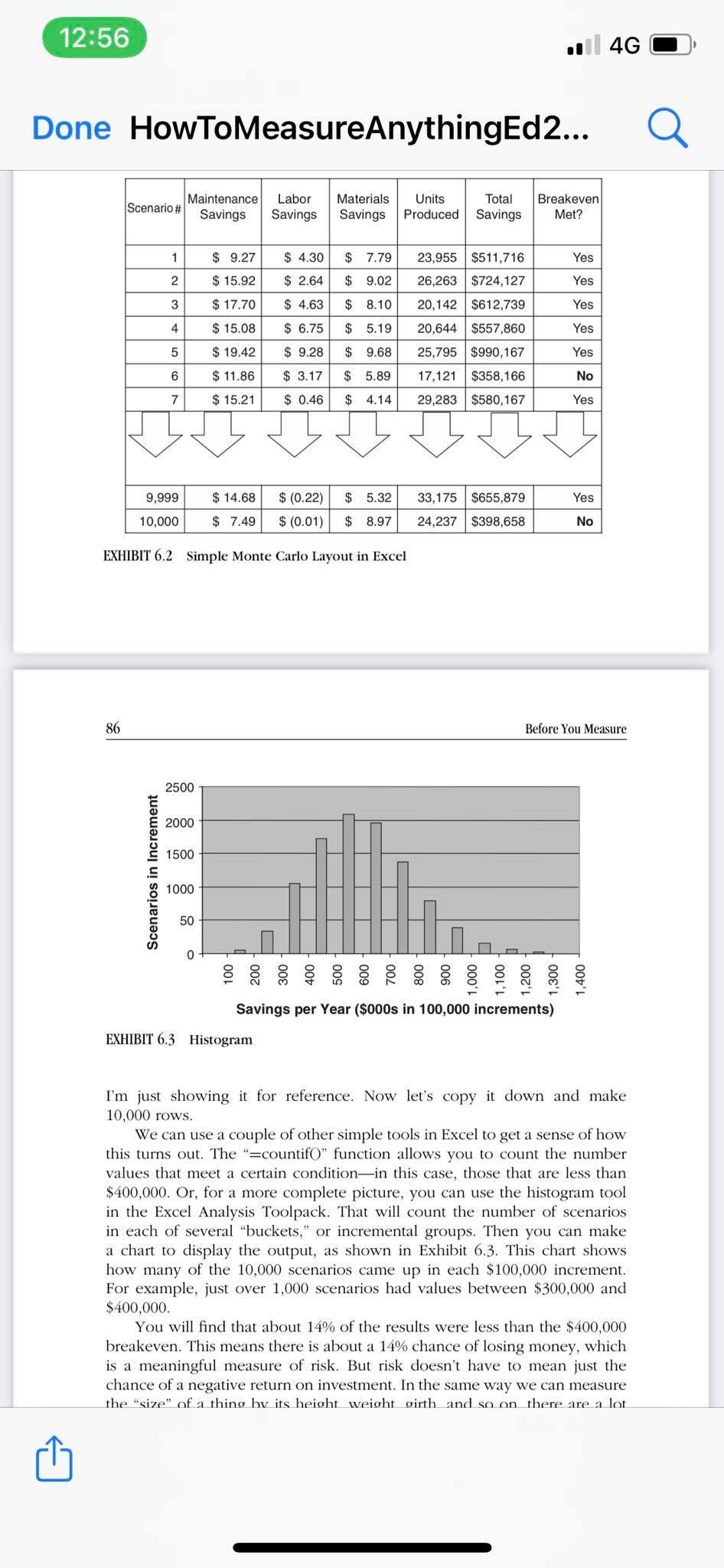
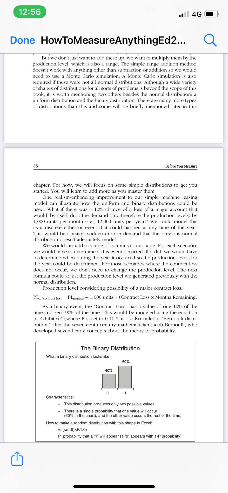
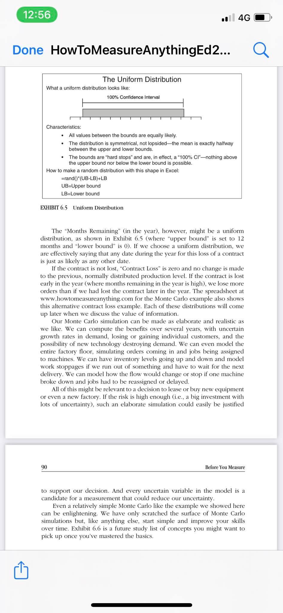
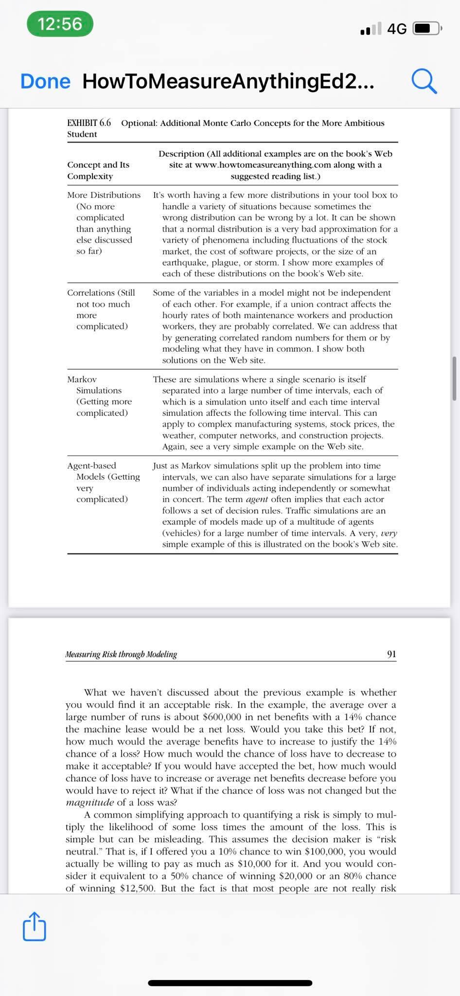
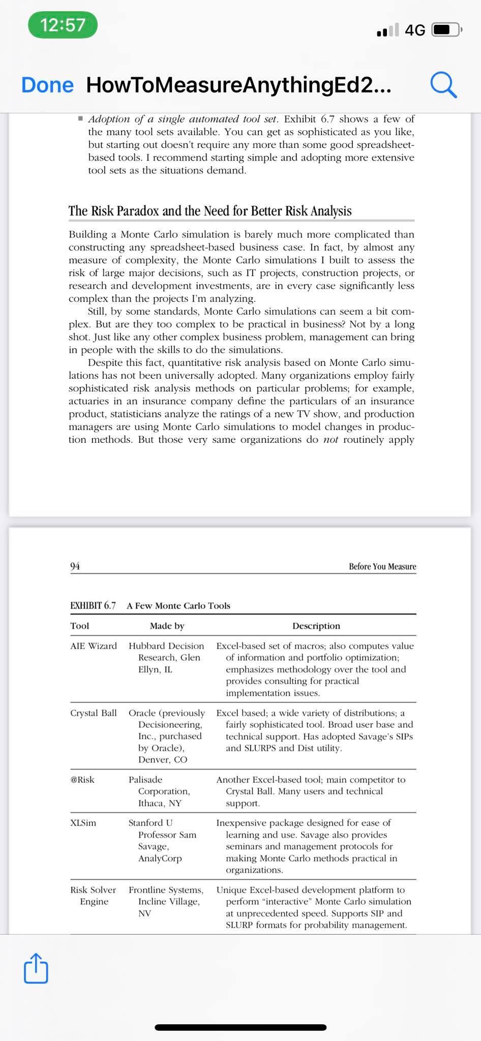
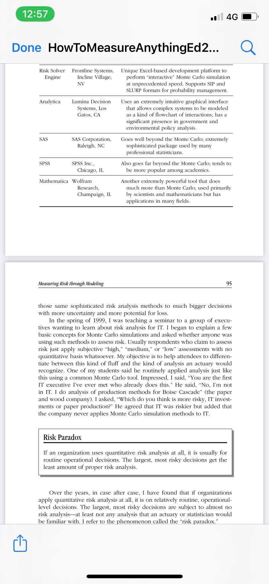
12:55 .4G Done HowToMeasureAnythingEd2... CHAPTER 6 Measuring Risk through Modeling It is better to be approximately right than to be precisely wrong. -Warren Buffett We e've defined the difference between uncertainty and risk. Initially, measuring uncertainty is just a matter of putting our calibrated ranges or probabilities on unknown variables. Subsequent measurements reduce uncertainty about the quantity and, in addition, quantify the new state of uncertainty. As discussed in Chapter 4, risk is simply a state of uncertainty where some possible outcomes involve a loss of some kind. Generally, the implication is that the loss is something dramatic, not minor. But for our purposes, any loss will do. Risk is itself a measurement that has a lot of relevance on its own. But it is also a foundation of any other important measurement. As we will see in Chapter 7, risk reduction is the basis of computing the value of a measurement, which is in turn the basis of selecting what to measure and how to measure it. Remember, if a measurement matters to you at all, it is because it must inform some decision that is uncertain and has negative consequences if it turns out wrong. This chapter will discuss a basic tool for almost any kind of risk analysis and some surprising observations you might make when you start using this tool. But first, we need to separate from this some popular schemes that are often used to measure risk but really offer no insight. How Not to Measure Risk What many organizations do to "measure" risk is not very enlightening. The methods I propose for assessing risk would be familiar to an actuary, statistician, or financial analyst. But some of the most popular methods for 79 80 Before You Measure measuring risk look nothing like what an actuary might be familiar with. Many organizations simply say a risk is "high," "medium," or "low." Or perhaps they rate it on a scale of 1 to 5. When I find situations like this, I sometimes ask how much "medium" risk really is. Is a 5% chance of losing more than $5 million a low, medium, or high risk? Nobody knows. Is a medium-risk investment with a 15% return on investment better or worse than a high-risk investment with a 50% return? Again, nobody knows because the statements themselves are ambiguous. Researchers have shown, in fact, that such ambiguous labels don't help the decision maker at all and actually add an error of their own. They 12:55 4G Done HowToMeasureAnythingEd2... Researchers have shown, in fact, that such ambiguous labels don't help the decision maker at all and actually add an error of their own. They add imprecision by forcing a kind of rounding error that, in practice, gives the same score to hugely different risks. Worse yet, in my 2009 book, The Failure of Risk Management, I show that users of these methods tend to cluster responses in a way that magnifies this effect2 (more on this in Chapter 12). In addition to these problems, the softer risk "scoring" methods man- agement might use make no attempt to address the typical human biases discussed in Chapter 5. Most of us are systematically overconfident and will tend to underestimate uncertainty and risks unless we avail ourselves of the training that can offset such effects. To illustrate why these sorts of classifications are not as useful as they could be, I ask attendees in seminars to consider the next time they have to write a check (or pay over the Web) for their next auto or homeowner's insurance premium. Where you would usually see the "amount" field on the check, instead of writing a dollar amount, write the word "medium" and see what happens. You are telling your insurer you want a "medium" amount of risk mitigation. Would that make sense to the insurer in any meaningful way? It probably doesn't to you, either. It is true that many of the users of these methods will report that they feel much more confident in their decisions as a result. But, as we will see in Chapter 12, this feeling should not be confused with evidence of effectiveness. We will learn that studies have shown that it is very possible to experience an increase in confidence about decisions and forecasts without actually improving things or even making them worse. For now, just know that there is apparently a strong placebo effect in many decision analysis and risk analysis methods. Managers need to start to be able to tell the difference between feeling better about decisions and actually having better track records over time. There must be measured evidence that decisions and forecasts actually improved. Unfortunately, risk analysis or risk management or decision analysis in general-rarely has a performance metric of its own.3 The good news is that some methods have been measured, and they show a real improvement. Measuring Risk through Modeling 81 Real Risk Analysis: The Monte Carlo Using ranges to represent your uncertainty instead of unrealistically precise point values clearly has advantages. When you allow yourself to use ranges and probabilities, you don't really have to assume anything you don't know for a fact. But precise values have the advantage of being simple to add, subtract, multiply, and divide in a spreadsheet. So how do we add, subtract, multiply, and divide in a spreadsheet when we have no exact values, only ranges? Fortunately, there is a practical, proven solution, and it can be performed on any modern personal computer. One of our measurement mentors, Enrico Fermi, was an early user of what was later called a "Monte Carlo simulation." A Monte Carlo simulation uses a computer to generate a large number of scenarios based on prob- abilities for inputs. For each scenario, a specific value would be randomly generated for each of the unknown variables. Then these specific values would go into a formula to compute an output for that single scenario. This process usually goes on for thousands of scenarios. 12:55 .4G Done HowToMeasureAnythingEd2... process usually goes on for thousands of scenarios. Fermi used Monte Carlo simulations to work out the behavior of large numbers of neutrons. In 1930, he knew that he was working on a problem that could not be solved with conventional integral calculus. But he could work out the odds of specific results in specific conditions. He realized that he could, in effect, randomly sample several of these situations and work out how neutrons would behave in a system. In the 1940s and 1950s, several mathematicians-most famously Stanislaw Ulam, John von Neumann, and Nicholas Metropolis-continued to work on similar problems in nuclear physics and started using computers to generate the random scenarios. This time they were working on the atomic bomb for the Manhattan Project and, later, the hydrogen bomb at Los Alamos. At the suggestion of Metropolis, Ulam named this computer-based method of generating random scenarios after Monte Carlo, a famous gambling hotspot, in honor of Ulam's uncle, a gambler. What Fermi begat, and what was later reared by Ulam, von Neumann, and Metropolis, is today widely used in business, government, and research. A simple application of this method is working out the return on an investment when you don't know exactly what the costs and benefits will be. Apparently, it is not obvious to some that uncertainty about the costs and benefits of some new investment is really the basis of that investment's risk. I once met with the chief information officer (CIO) of an investment firm in Chicago to talk about how the company can measure the value of information technology (IT). She said that they had a "pretty good handle on how to measure risk" but "I can't begin to imagine how to measure benefits." On closer look, this is a very curious combination of positions. 82 Before You Measure She explained that most of the benefits the company attempts to achieve in IT investments are improvements in basis points (1 basis point = 0.01% yield on an investment)-the return the company gets on the investments. it manages for clients. The firm hopes that the right IT investments can facilitate a competitive advantage in collecting and analyzing information that affects investment decisions. But when I asked her how the company came up with a value for the effect on basis points, she said staffers "just pick a number." In other words, as long as enough people are willing to agree on (or at least not too many object to) a particular number for increased basis points, that's what the business case is based on. While it's possible this number is based on some experience, it was also clear that she was more uncertain about this benefit than any other. But if this was true, how was the company measuring risk? Clearly, it was a strong possibility that the firm's largest risk in new IT, if it was measured, would be the firm's uncertainty about this benefit. She was not using ranges to express her uncertainty about the basis point improvement, so she had no way to incorporate this uncertainty into her risk calculation. Even though she felt confident the firm was doing a good job on risk analysis, she wasn't really doing any risk analysis at all. She was, in fact, merely experiencing the previously mentioned placebo effect from one of the ineffectual risk "scoring" methods. In fact, all risk in any project investment ultimately can be expressed by one method: the ranges of uncertainty on the costs and benefits and probabilities on events that might affect them. If you know precisely the amount and timing of every cost and benefit (as is implied by traditional 12:55 .4G Done HowToMeasureAnythingEd2... amount and timing of every cost and benefit (as is implied by traditional business cases based on fixed point values), you literally have no risk. There is no chance that any benefit would be lower or cost would be higher than you expect. But all we really know about these things is the range, not exact points. And because we only have broad ranges, there is a chance we will have a negative return. That is the basis for computing risk, and that is what the Monte Carlo simulation is for. An Example of the Monte Carlo Method Risk This is an extremely basic example of a Monte Carlo simulation for people who have never worked with it before but have some familiarity with the Excel spreadsheet. If you have worked with a Monte Carlo tool before, you probably can skip these next few pages. Let's say you are considering leasing a new machine for one step in a manufacturing process. The one-year lease is $400,000 with no option for early cancellation. So if you aren't breaking even, you are still stuck with it for the rest of the year. You are considering signing the contract because Measuring Risk through Modeling 83 you think the more advanced device will save some labor and raw materials and because you think the maintenance cost will be lower than the existing process. Your calibrated estimators gave the next ranges for savings in mainte- nance, labor, and raw materials. They also estimated the annual production levels for this process. Maintenance savings (MS): $10 to $20 per unit Labor savings (LS): -$2 to $8 per unit Raw materials savings (RMS): $3 to $9 per unit Production level (PL): 15,000 to 35,000 units per year Annual lease (breakeven): $400,000 Now you compute your annual savings very simply as: Annual Savings = (MS + LS + RMS) X PL Admittedly, this is an unrealistically simple example. The production levels could be different every year, perhaps some costs would improve further as experience with the new machine improved, and so on. But we've deliberately opted for simplicity over realism in this example. If we just take the midpoint of each of these ranges, we get Annual Savings ($15+$3+ $6) x 25,000 = $600,000 It looks like we do better than the required breakeven, but there are uncertainties. So how do we measure the risk of this lease? First, let's define risk for this context. Remember, to have a risk, we have to have uncertain future results with some of them being a quantified loss. One way of looking at risk would be the chance that we don't break even that is, we don't save enough to make up for the $400,000 lease. The farther the savings undershoot the lease, the more we have lost. The $600,000 is the amount we save if we just choose the midpoints of each uncertain variable. How do we compute what that range of savings really is and, thereby, compute the chance that we don't break even? 12:56 .4G Done HowToMeasureAnythingEd2... the chance that we don't break even? Since these aren't exact numbers, usually we can't just do a single cal- culation to determine whether we met the required savings. Some methods allow us to compute the range of the result given the ranges of inputs un- der some limited conditions, but in most real-life problems, those conditions don't exist. As soon as we begin adding and multiplying different types of distributions, the problem usually becomes what a mathematician would call "unsolvable" or "having no solution." This is exactly the problem the physi- cists working on atomic fission ran into. To resolve this problem, Monte Carlo simulations use a brute-force approach made possible with ers. We randomly pick a bunch of exact values-thousands-according to 84 Before You Measure the ranges we prescribed and compute a large number of exact values. Then we use those randomly chosen values to compute a single result. Af- ter thousands of possible results are calculated, the probabilities of different results can be estimated. In this example, each scenario is a set of randomly generated values for labor savings, maintenance savings, and so on. After each set is generated, those values are used in the annual savings calculation. Some of the annual savings results will be higher than $600,000 and some will be lower. Some will even be lower than the $400,000 required to break even. After thousands of scenarios are generated, we can determine how likely it is that the lease will be a net gain. You can run a Monte Carlo simulation easily with Excel on a PC, but we need a bit more information than just the 90% confidence interval (CI) for each of the variables. We also need the shape of the distribution. Some shapes are more appropriate for certain values than other shapes. One that is often used with the 90% CI is the well-known "normal" distribution. The normal distribution is the familiar-looking bell curve where the probable outcomes are bunched near the middle but trail off to ever less likely values in both directions. (See Exhibit 6.1.) With the normal distribution, I will briefly mention a related concept called the standard deviation. People don't seem to have an intuitive The Normal Distribution What a normal distribution looks like: 90% Confidence Interval Characteristics: Values near the middle are more likely than values farther away. The distribution is symmetrical, not lopsided-the mean is exactly halfway between the upper and lower bounds of a 90% CI. The ends trail off indefinitely to ever more unlikely values, but there is no "hard stop"; a value far outside of a 90% CI is possible but not likely. How to make a random distribution with this shape in Excel: =norminv(rand(), A, B) A=mean = (90% CI upper bound + 90% CI lower bound)/2 and 12:56 .4G Done HowToMeasureAnythingEd2... The Normal Distribution What a normal distribution looks like: 90% Confidence Interval. Characteristics: Values near the middle are more likely than values farther away. The distribution is symmetrical, not lopsided-the mean is exactly halfway between the upper and lower bounds of a 90% CI. The ends trail off indefinitely to ever more unlikely values, but there is no "hard stop"; a value far outside of a 90% CI is possible but not likely. How to make a random distribution with this shape in Excel: =norminv(rand(), A, B) A=mean = (90% CI upper bound + 90% CI lower bound)/2 and B="standard deviation" =(90% CI upper bound - 90% CI lower bound)/3.29 EXHIBIT 6.1 Normal Distribution Measuring Risk through Modeling 85 understanding of standard deviation, and because it can be replaced by a calculation based on the 90% CI (which people do understand intuitively), I won't focus on it here. Exhibit 6.1 shows that there are 3.29 standard deviations in one 90% CI, so we just need to make the conversion. For our problem, we can just make a random number generator in a spreadsheet for each of our ranges. Following the instructions in Exhibit 6.1, we can generate random numbers for Maintenance savings with the Excel formula: = norminv(rand(), 15, (2010)/3.29) Likewise, we follow the instructions in Exhibit 6.1 for the rest of the ranges. Some people might prefer using the random number generator in the Excel Analysis Toolpack, and you should feel free to experiment with it. I'm showing this formula in Exhibit 6.2 for a bit more of a hands-on approach. (Download this spreadsheet from www.howtomeasureanything.com.) We arrange the variables in columns as shown in Exhibit 6.2. The last two columns are just the calculations based on all the previous columns. The Total Savings column is the formula for annual savings (shown ear- lier) based on the numbers in each particular row. For example, sce- nario 1 in Exhibit 6.2 shows its Total Savings as ($9.27 + $4.30 + $7.79) X 23,955 $511,716. You don't really need the "Breakeven Met?" column; Scenario # Maintenance Labor Materials Units Total Savings Savings Savings Produced Savings Breakeven Met? 1 Yes 2 $9.27 $4.30 $ 7.79 23,955 $511,716 $15.92 $2.64 $9.02 26,263 $724,127 $4.63 $8.10 20,142 $612,739 Yes 3 $ 17.70 Yes 12:56 4G Done HowToMeasureAnythingEd2... Total Scenario # Maintenance Labor Materials Units Savings Savings Savings Produced Savings Breakeven Met? 1 $9.27 $4.30 $ 7.79 23,955 $511,716 Yes 2 $15.92 $2.64 $9.02 26,263 $724,127 Yes 3 $17.70 $4.63 $ 8.10 20,142 $612,739 Yes 4 $15.08 20,644 $557,860 Yes $6.75 $ 5.19 $9.28 $9.68 5 $ 19.42 Yes 6 $11.86 $3.17 $5.89 $ 0.46 $4.14 25,795 $990,167 17,121 $358,166 29,283 $580,167 No 7 $15.21 Yes $655,879 Yes 9,999 10,000 $14.68 $ (0.22) $ 5.32 $7.49 $ (0.01) $8.97 33,175 24,237 $398,658 No EXHIBIT 6.2 Simple Monte Carlo Layout in Excel 86 Before You Measure Scenarios in Increment 2500 2000 1500 1000 50 0 P ,100 1,200 1,300 1,400 Savings per Year ($000s in 100,000 increments) EXHIBIT 6.3 Histogram I'm just showing it for reference. Now let's copy it down and make 10,000 rows. We can use a couple of other simple tools in Excel to get a sense of how this turns out. The "=countifO" function allows you to count the number values that meet a certain condition in this case, those that are less than $400,000. Or, for a more complete picture, you can use the histogram tool in the Excel Analysis Toolpack. That will count the number of scenarios in each of several "buckets," or incremental groups. Then you can make a chart to display the output, as shown in Exhibit 6.3. This chart shows how many of the 10,000 scenarios came up in each $100,000 increment. For example, just over 1,000 scenarios had values between $300,000 and $400,000. You will find that about 14% of the results were less than the $400,000 breakeven. This means there is about a 14% chance of losing money, which is a meaningful measure of risk. But risk doesn't have to mean just the chance of a negative return on investment. In the same way we can measure the "size" of a thing by its height weight girth and so on there are a lot. 12:56 .4G Done HowToMeasureAnythingEd2... You will find that about 14% of the results were less than the $400,000 breakeven. This means there is about a 14% chance of losing money, which is a meaningful measure of risk. But risk doesn't have to mean just the chance of a negative return on investment. In the same way we can measure the "size" of a thing by its height, weight, girth, and so on, there are a lot of useful measures of risk. Further examination shows that there is a 3.5% chance that the factory will lose more than $100,000 per year instead of saving money. However, generating no revenue at all is virtually impossible. This is what we mean by "risk analysis." We have to be able to compute the odds of various levels of losses. If you are truly measuring risk, this is what you can do. Again, for a spreadsheet example of this Monte Carlo problem, see the Web site at www.howtomeasureanything.com. A shortcut can apply in some situations. If we had all normal distribu- tions and we simply wanted to add or subtract ranges-such as a simple list of costs and benefits we might not have to run a Monte Carlo simulation. Measuring Risk through Modeling 87 If we just wanted to add up the three types of savings in our example, we can use a simple calculation. Use these six steps to produce a range: 1. Subtract the midpoint from the upper bound for each of the three cost savings ranges: in this example, $20-$15= $5 for maintenance savings; we also get $5 for labor savings and $3 for materials savings. 2. Square each of the values from the last step: $5 squared is $25, and so on. 3. Add up the results: $25 + $25 + $9 = $59. 4. Take the square root of the total: $59.5 = $7.68. 5. Total up the means: $15 + $3+ $6= $24. 6. Add and subtract the result from step 4 from the sum of the means to get the upper and lower bounds of the total, or $24+ $7.68 for the upper bound, $24 - $7.68 = $16.32 for the lower bound. $31.68 So the 90% CI for the sum of all three 90% CIs for maintenance, labor, and materials is $16.32 to $31.68. In summary, the range interval of the total is equal to the square root of the sum of the squares of the range intervals. (Note: If you are already familiar with the 90% CI from a basic stats text or have already read ahead to Chapter 9, keep in mind that $7.68 is not the standard deviation. $7.68 is the difference between the midpoint of the range and either of the bounds of a 90% CI, which is 1.645 standard deviations.) You might see someone attempting to do something similar by adding up all the "optimistic" values for an upper bound and "pessimistic" values for the lower bound. This would result in a range of $11 to $37 for these three Cls, which slightly exaggerates the 90% CI. When this calculation is done with a business case of dozens of variables, the exaggeration of the range becomes too significant to ignore. It is like thinking that rolling a bucket of six-sided dice will produce all 1s or all 6s. Most of the time, we get a combination of all the values, some high, some low. Using all optimistic values for the optimistic case and all pessimistic values for the pessimistic case is a common error and no doubt has resulted in a large number of misinformed decisions. The simple method I just showed works perfectly well when you have a set of 90%; CIs you would like to add up. But we don't just want to add these up, we want to multiply them by the production level, which is also a range. The simple range addition method doesn't work with anything other than subtraction or addition so we would 12:56 .4G Done HowToMeasureAnythingEd2... But we don't just want to add these up, we want to multiply them by the production level, which is also a range. The simple range addition method doesn't work with anything other than subtraction or addition so we would need to use a Monte Carlo simulation. A Monte Carlo simulation is also required if these were not all normal distributions. Although a wide variety of shapes of distributions for all sorts of problems is beyond the scope of this book, it is worth mentioning two others besides the normal distribution: a uniform distribution and the binary distribution. There are many more types of distributions than this and some will be briefly mentioned later in this 88 Before You Measure chapter. For now, we will focus on some simple distributions to get you started. You will learn to add more as you master them. One realism-enhancing improvement to our simple machine leasing model can illustrate how the uniform and binary distributions could be used. What if there was a 10% chance of a loss of a major account that would, by itself, drop the demand (and therefore the production levels) by 1,000 units per month (i.e., 12,000 units per year)? We could model this as a discrete either/or event that could happen at any time of the year. This would be a major, sudden drop in demand that the previous normal distribution doesn't adequately model. We would just add a couple of columns to our table. For each scenario, we would have to determine if this event occurred. If it did, we would have to determine when during the year it occurred so the production levels for the year could be determined. For those scenarios where the contract loss does not occur, we don't need to change the production level. The next formula could adjust the production level we generated previously with the normal distribution: Production level considering possibility of a major contract loss: PLw/contract loss =PLnormal 1,000 units x (Contract Loss x Months Remaining) As a binary event, the "Contract Loss" has a value of one 10% of the time and zero 90% of the time. This would be modeled using the equation in Exhibit 6.4 (where P is set to 0.1). This is also called a "Bernoulli distri- bution," after the seventeenth-century mathematician Jacob Bernoulli, who developed several early concepts about the theory of probability. The Binary Distribution What a binary distribution looks like: 60% 40% 0 1 Characteristics: This distribution produces only two possible values. There is a single probability that one value will occur (60% in the chart), and the other value occurs the rest of the time. How to make a random distribution with this shape in Excel: =if(rand()