refer to the attachment
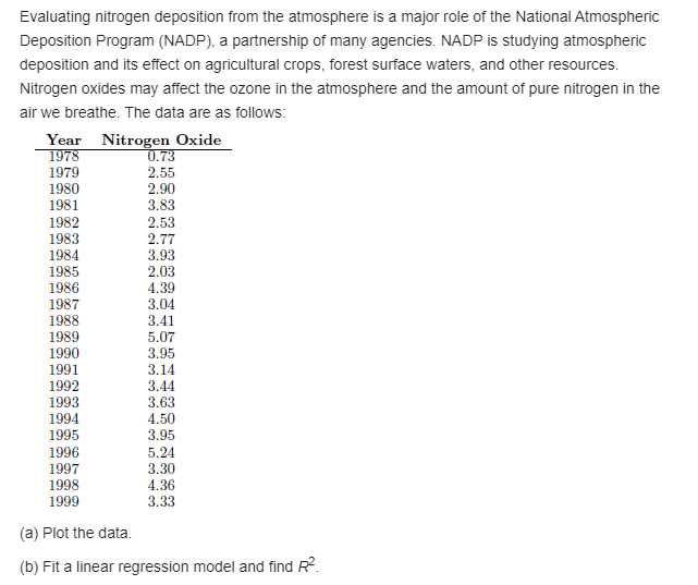
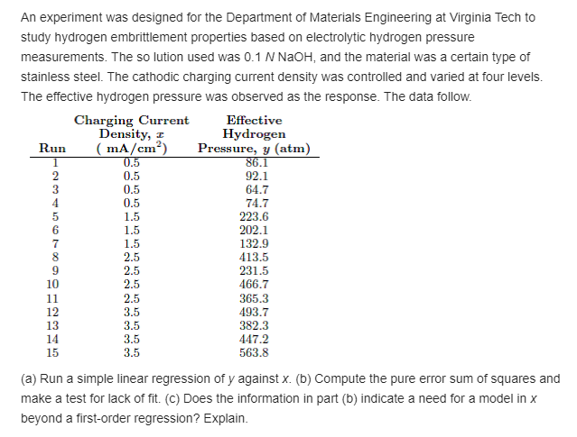
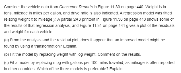
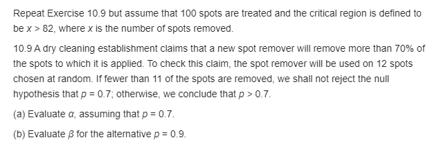
Evaluating nitrogen deposition from the atmosphere is a major role of the National Atmospheric Deposition Program (NADF'), a partnership of many agencies. NADP is studying atmospheric deposition and its effect on agncuitural crops, forest surface waters, and other resources. Nitrogen oxides may.r affect the ozone in the atmosphere and the amount of pure nitrogen in the airwe breathe. The data are as follows: Year Nitrogen Oxide. 1973 U 33 1979 3.55 1939 3.99 1931 3.33 1933 3.53 1933 3.77 1934 3.93 1935 3.93 1935 4.39 1937 3.94 1933 3.41 1939 5.97 1999 3.95 1991 3.14 1993 3.44 1993 3.93 1994 4.59 1995 3.95 1995 5.34 1997 3.39 1993 4.35 1999 3.33 {3) Plot the data. to} Fit a linear regression model and nd R2. \f\f\fAn experiment was designed for the Department of Materials Engineering at Virginia Tech to study hydrogen embriltlement properties based on electrolytic hydrogen pressure measurements. The so Iuljon used was [11 N NaDH. and the material was a certain type of stainless steel. The cathodic charging current density was controlled and varied at four levels. The effective hydrogen pressure was observed as the response. The data follow. Charging Curr-t. EfFective Density, :3. Hydrogen Run { rnAfcmE} Pressure, 1: [atm] 1 5.5 35.1 2 l[L5 92.1 3 115 54.'i'r 4 l[L5 34.7 5 1.5 223.5 5 1.5 252.1 \"J? 1.5 132.9 8 2.5 413.5 9 2.5 231.5 15 2.5 455.'ir 11 2.5 355.3 12 3.5 433.1r 13 3.5 332.3 14 3.5 44?.2 15 3.5 553.8 {a} Run a simple linear regression of y against 1.. {b} Compute the pure error sum of squares and make a test for laclt of lit. (c) Does the information in part (b} indicate a need for a model in x beyond a rstorder regression? Explain. Consider the vehicle data from Consumer Reports in Figure 11.3 on page 44D. Weight is in to ns, mileage in miles per gallon, and drive raljo is also indicated. A regression model was tted relating weight xto mileage y. A partial 3A3 printout in Figure 11.3(l on page 44o shows some of the results of that regression analysis, and Figure 11.31 on page 441 gives a plot of the residuals and weight for each vehicle. {a} From the analysis and the residual plot, does it appear that an improved model might be found by using a transformation? Explain. {h} Fitthe model by replacing weight 1with log weight. Comment on the results. {c} Fit a model by replacing mpg with gallons per 10D miles traveled, as mileage is often reported in other countries. 1I.I'I.I'hich of the three models is preferable? Explain. Repeat Exercise 10.9 but assume that 1oo spots are treated and the critical region is dened to he x :=- 32, where x is the number of spots removed. 10.9 i'itdriir cleaning establishment claims that a new spot remover will remove more than TFG'K: of the spots to which it is applied. To check; this claim, the spot remover will he used on 12 spots chosen at random. If fewer than 11 of the spots are removed, we shall not reject the null hypothesis that p = (1?; otherwise, we conclude that p :-~ [l]. {a} Evaluate o, assuming that p = (1?. in} Evaluate p for the altemaijve p = as
