Regression analysis can be used to test whether the market efficiently uses information in valuing stocks. Let return be the total return (measured in %) from holding a firm's stock over the four-year period from the end of 1990 to the end 1994. The efficient markets hypothesis (EMH) says that these returns should not be systematically related to information known in 1990. If firm characteristics known at the beginning of the period help to predict stock returns, then we could use this information in choosing stocks.

For 1990, let dkr be a firm's debt-to-capital ratio, let eps denote the earnings per share, let netinc denote the net income, and let salary denote total compensation for the CEO.

Using the data in Computer_Exercse_10.xlsx, please answer the following questions. Assume throughout that assumptions MLR.1-MLR.6 are satisfied.

1. Estimate the following regression: = 0 + 1 + 2 + 3ln () + 4ln() + by OLS and report results in the usual format. Are the slope coefficient individually statistically significant?

2. Interpret in words the estimate for 3

3. If a firms debt-to-capital ratio increases by 1.5 and, simultaneously, its earning per share increase by 4.5, what is the predicted change in returns (holding ln(netinc) and ln(salary) fixed)?

4. Compute the 90%, 95%, and 99% confidence intervals for the intercept. What do you conclude with respect to the following hypothesis: If everything else were equal to zero, the predicted (base) return would be 35%?

5. Evaluate the null hypothesis that 25 times the effect of the firm's debt-to-capital ratio is of the same magnitude as the effect of the CEOs log-salary. That is, test the following null hypothesis: 0: 251 = 4 Test the null hypothesis against the one-sided right-tailed alternative, at a 10% significance level.

6. Evaluate the null hypothesis that the effect of is 0.5 while at the same time (i.e. jointly) the effect of is zero. Let the significance level be 0.05.

7. Evaluate the EMH. That is, test whether the independent variables are jointly significant at a 1%, 5%, and 10% significance level. What can you conclude with respect to the EMH?

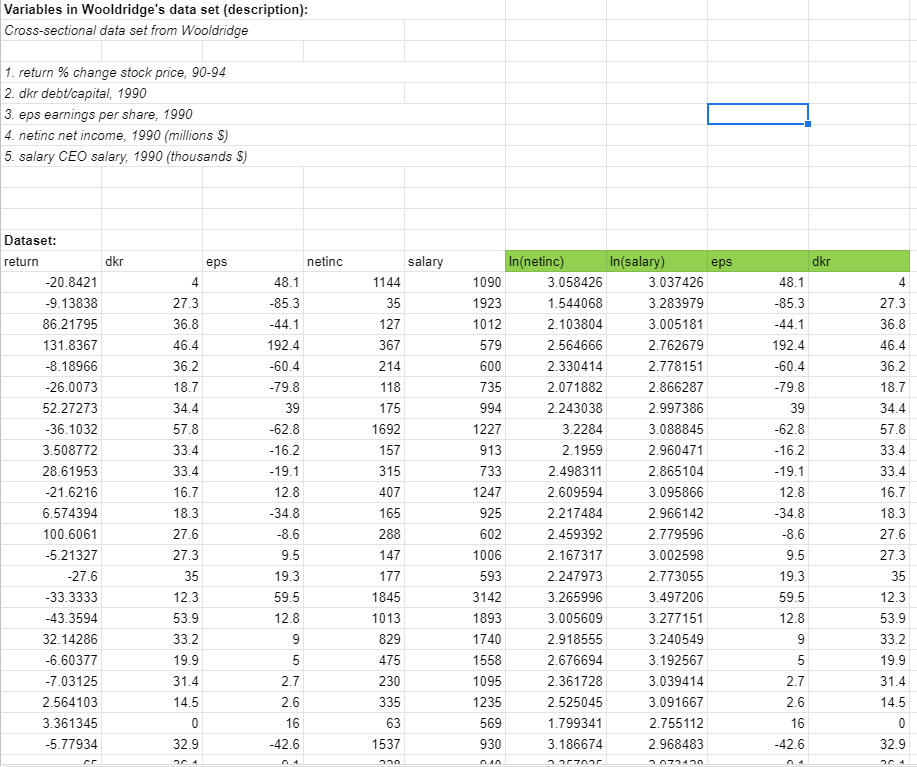
Variables in Wooldridge's data set (description): Cross-sectional data set from Wooldridge 1. return % change stock price, 90-94 2. dkr debt/capital, 1990 3. eps earnings per share, 1990 4. netinc net income, 1990 (millions $) 5. salary CEO salary, 1990 (thousands 5) dkr netinc salary eps dkr 4 1090 1923 1012 579 600 Dataset: return -20.8421 -9.13838 86.21795 131.8367 -8.18966 -26.0073 52.27273 -36.1032 3.508772 28.61953 -21.6216 6.574394 100.6061 -5.21327 -27.6 -33.3333 -43.3594 32.14286 -6.60377 -7.03125 2.564103 3.361345 -5.77934 eps 4 27.3 36.8 46.4 36.2 18.7 34.4 57.8 33.4 33.4 16.7 18.3 27.6 27.3 35 12.3 53.9 33.2 19.9 31.4 14.5 0 32.9 48.1 -85.3 -44.1 192.4 -60.4 -79.8 39 -62.8 -16.2 -19.1 12.8 -34.8 -8.6 9.5 19.3 59.5 12.8 9 5 2.7 2.6 16 -42.6 1144 35 127 367 214 118 175 1692 157 315 407 165 288 147 177 1845 1013 829 475 230 335 63 1537 735 994 1227 913 733 1247 925 602 1006 593 3142 1893 1740 1558 1095 1235 569 930 In(netinc) 3.058426 1.544068 2.103804 2.564666 2.330414 2.071882 2.243038 3.2284 2.1959 2.498311 2.609594 2.217484 2.459392 2.167317 2.247973 3.265996 3.005609 2.918555 2.676694 2.361728 2.525045 1.799341 3.186674 In(salary) 3.037426 3.283979 3.005181 2.762679 2.778151 2.866287 2.997386 3.088845 2.960471 2.865104 3.095866 2.966142 2.779596 3.002598 2.773055 3.497206 3.277151 3.240549 3.192567 3.039414 3.091667 2.755112 2.968483 48.1 -85.3 -44.1 192.4 -60.4 -79.8 39 -62.8 -16.2 -19.1 12.8 -34.8 -8.6 9.5 19.3 59.5 12.8 9 5 2.7 2.6 16 -42.6 27.3 36.8 46.4 36.2 18.7 34.4 57.8 33.4 33.4 16.7 18.3 27.6 27.3 35 12.3 53.9 33.2 19.9 31.4 14.5 6 0 32.9 4 Variables in Wooldridge's data set (description): Cross-sectional data set from Wooldridge 1. return % change stock price, 90-94 2. dkr debt/capital, 1990 3. eps earnings per share, 1990 4. netinc net income, 1990 (millions $) 5. salary CEO salary, 1990 (thousands 5) dkr netinc salary eps dkr 4 1090 1923 1012 579 600 Dataset: return -20.8421 -9.13838 86.21795 131.8367 -8.18966 -26.0073 52.27273 -36.1032 3.508772 28.61953 -21.6216 6.574394 100.6061 -5.21327 -27.6 -33.3333 -43.3594 32.14286 -6.60377 -7.03125 2.564103 3.361345 -5.77934 eps 4 27.3 36.8 46.4 36.2 18.7 34.4 57.8 33.4 33.4 16.7 18.3 27.6 27.3 35 12.3 53.9 33.2 19.9 31.4 14.5 0 32.9 48.1 -85.3 -44.1 192.4 -60.4 -79.8 39 -62.8 -16.2 -19.1 12.8 -34.8 -8.6 9.5 19.3 59.5 12.8 9 5 2.7 2.6 16 -42.6 1144 35 127 367 214 118 175 1692 157 315 407 165 288 147 177 1845 1013 829 475 230 335 63 1537 735 994 1227 913 733 1247 925 602 1006 593 3142 1893 1740 1558 1095 1235 569 930 In(netinc) 3.058426 1.544068 2.103804 2.564666 2.330414 2.071882 2.243038 3.2284 2.1959 2.498311 2.609594 2.217484 2.459392 2.167317 2.247973 3.265996 3.005609 2.918555 2.676694 2.361728 2.525045 1.799341 3.186674 In(salary) 3.037426 3.283979 3.005181 2.762679 2.778151 2.866287 2.997386 3.088845 2.960471 2.865104 3.095866 2.966142 2.779596 3.002598 2.773055 3.497206 3.277151 3.240549 3.192567 3.039414 3.091667 2.755112 2.968483 48.1 -85.3 -44.1 192.4 -60.4 -79.8 39 -62.8 -16.2 -19.1 12.8 -34.8 -8.6 9.5 19.3 59.5 12.8 9 5 2.7 2.6 16 -42.6 27.3 36.8 46.4 36.2 18.7 34.4 57.8 33.4 33.4 16.7 18.3 27.6 27.3 35 12.3 53.9 33.2 19.9 31.4 14.5 6 0 32.9 4