RELEVANT ANSWERS ONLY!!! THESE ARE 1 QUESTION

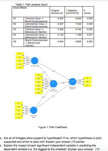
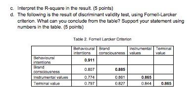
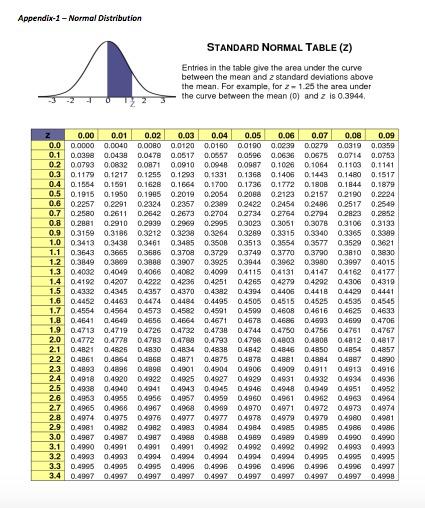
Question 4 (30 Points): The following is the result of a PLS-SEM on a model of Shopping Values, Brand Consciousness and Behavioral Intention in purchasing luxury goods Table 1. Path analysis result Direct Effects P Original T Statistics Sample (O) (OSTDEVI 0.350 4.654 Values H1 0.000 H2 0.567 7564 0.000 ER |F | | H3 0.358 4.162 0.000 Terminal Value -> Brard Consciousness Instrumental Value -> Brand Consciousness Terminal Value -> Behavioural Intention Instrumental Value -> Behavioural Intention Brand Consciousness -> Behavioural Interton H4 0.124 1.196 0.231 H5 0.404 3.665 0.000 THE SEM The Figure 1. Path Coefficient a. Are all of linkages show support to hypotheses? If no, which hypotheses is (are) supported and which is (are) not? Explain your answer (10 points) . Explain the impact of each significant independent variable in predicting the dependent variable (i.e. the biggest to the smallest). Explain your answer. (10 c. Interpret the R-square in the result. (5 points) d. The following is the result of discriminant validity test, using Fornell-Larcker criterion. What can you conclude from the table? Support your statement using numbers in the table. (5 points) Table 2 Fornell Larcker Criterion Behavioural Brand Instrumental Teminal intentions consciousness values value 0.911 Behavioural Intentions Brand conscious Instrumental values Terminal value 0.807 0.885 0.774 0.797 0.881 0.827 0.865 0.844 0.865 Appendix-1 - Normal Distribution STANDARD NORMAL TABLE() Entries in the table give the area under the curve between the mean and a standard deviations above the mean. For example, for 2 -1.25 the area under the curve between the mean (O) and z is 0.3944, Z 0.00 0.01 0.02 0.03 0.04 0.05 0.06 0.07 0.08 0.09 0.0 0.0000 0.0040 0.0080 0.0120 0,0150 0.0190 0.0239 0.0279 0.0319 0.0359 0.1 0.0300 0.0438 0.0478 0.0517 0.0557 0.0596 0.0636 0.0675 0.0714 0.0753 0.2 0.0793 0.0832 0.0871 0.0910 0.0948 0.0987 0.1026 0.1054 0.1103 0.1141 0.3 0.1179 0.1217 0.1255 0.1203 0.1331 0.1368 0.1405 0.1443 0.1480 0.1517 0.4 0.1554 0.1591 0.1628 0.1664 0.1700 0.1736 0.1772 0.1808 0.1844 0.1879 0.5 0.1915 0.1950 0.1995 0.2019 0.2054 0.2088 0.2123 0.2157 0.2190 0.2224 0.6 0.2257 0.2291 0.2324 0.2357 0.2389 0.2422 0.2154 0.2486 0.2517 0.2549 0.7 0.2580 0.2611 0.2642 0.2673 0.2704 0.2734 0.2754 0.2794 0.2923 0.2852 0.8 0.2881 0.2910 0.2939 0.2909 0.2995 0.3023 0.3051 0.3078 0.3106 0.3133 0.9 0.3159 0.3186 0.3212 0.3238 0.3264 0.3289 0.3315 0.3340 0.3365 0.3389 1.0 0.3413 0.3438 0.3461 0.3485 0.3508 03513 0.3554 0.3577 0.3529 0.3621 1.1 0.3643 0.3655 0.3686 0.3709 0.3729 0.3749 0.3770 0.3790 0.3810 0.3830 12 0.3849 0.3889 0.3888 0.3907 0.3925 0.3944 0.3962 0.3980 0.3997 0.4015 1.3 0.4032 0.4049 0.4066 0.4082 0.4099 0.4115 0.4131 0.4147 0.4162 0.4177 1.4 0.4192 0.4207 0.4222 0.4236 0.4251 0.4265 0.4279 0.4292 0.4306 0.4319 1.5 0.4112 0.4345 0.4357 0.4370 0.4382 0.4394 0,4406 0.4418 0.4429 0.4441 1.6 0.4452 0.4463 0.4474 0.4484 0.4495 0.4505 0.4515 0.4525 0.4535 0.4545 1.7 0.4554 9.4564 0.4573 0.4582 0,4591 0.4599 0.4608 0.4625 0,4633 1.8 0.4641 0.4640 0.4656 0.4664 0.4671 0.4678 0.4686 0.4693 0.4609 0.4706 1.9 0.4713 0.4719 0.4726 0.4732 0.4730 0.4744 0.4750 0.4756 0.4761 0.4767 2.0 0.4772 0.4778 0.4783 0.4789 0.4793 0.4798 0.4803 0.4808 0.4012 0.4817 2.1 0.4821 0.4825 0.4830 0.4834 0,4838 0.4842 0.4846 0.4850 0.4854 0.4857 22 0.4861 0.4864 0.4868 0.4871 0.4875 0.4878 0.4881 0.4894 0.4887 0.4890 2.3 0.4893 0.4896 0.4890 0.4001 0.4904 04906 0,4909 0.4911 0.4913 0.4916 2.4 0.4918 0.4920 0.4922 0.4925 0.4927 0.4929 0.4931 0.4932 0.4934 0.4936 2.5 0.4938 9.4940 0.4941 0.4943 0,4945 0.4946 0.4948 0.4949 0.4951 0.4952 2.6 0.4963 0.4955 0.4956 0.4967 0.4959 0.4960 0.4961 0.4962 0.4963 0.4964 2.7 0.4965 0.4966 0.4967 0.46 0.4989 0.4970 0.4971 0.4972 0.4973 0.4974 2.8 0.4974 0.4975 0.4976 0.4977 0.4977 0.4978 0,4979 0.4979 0.4980 0.4981 2.9 0.4981 0.4982 0.4982 0.4083 0.4984 0.4984 0.4985 0.4985 0.4988 0.4986 30 0.4987 37 0.4987 0.48 0.4998 0.4989 0.4999 0.4000 0.4990 3.1 0.4990 0.4991 0.4991 0.4991 0.4992 0.4992 0.4992 0.4992 0.4993 0.4993 3.2 0.4993 0.4993 0.4994 0.4994 0.4994 0.4994 0.4904 0.4995 0.4995 0,4995 3.3 0.4995 0.4095 0.4995 0.400 0.4996 0.4996 0.4996 0.4996 0.4906 0.4907 3.4 0.4997 0.4997 0.4997 0.4897 0.4997 0.4997 0.4997 0.4997 0.4997 0.4999 0.4616 Question 4 (30 Points): The following is the result of a PLS-SEM on a model of Shopping Values, Brand Consciousness and Behavioral Intention in purchasing luxury goods Table 1. Path analysis result Direct Effects P Original T Statistics Sample (O) (OSTDEVI 0.350 4.654 Values H1 0.000 H2 0.567 7564 0.000 ER |F | | H3 0.358 4.162 0.000 Terminal Value -> Brard Consciousness Instrumental Value -> Brand Consciousness Terminal Value -> Behavioural Intention Instrumental Value -> Behavioural Intention Brand Consciousness -> Behavioural Interton H4 0.124 1.196 0.231 H5 0.404 3.665 0.000 THE SEM The Figure 1. Path Coefficient a. Are all of linkages show support to hypotheses? If no, which hypotheses is (are) supported and which is (are) not? Explain your answer (10 points) . Explain the impact of each significant independent variable in predicting the dependent variable (i.e. the biggest to the smallest). Explain your answer. (10 c. Interpret the R-square in the result. (5 points) d. The following is the result of discriminant validity test, using Fornell-Larcker criterion. What can you conclude from the table? Support your statement using numbers in the table. (5 points) Table 2 Fornell Larcker Criterion Behavioural Brand Instrumental Teminal intentions consciousness values value 0.911 Behavioural Intentions Brand conscious Instrumental values Terminal value 0.807 0.885 0.774 0.797 0.881 0.827 0.865 0.844 0.865 Appendix-1 - Normal Distribution STANDARD NORMAL TABLE() Entries in the table give the area under the curve between the mean and a standard deviations above the mean. For example, for 2 -1.25 the area under the curve between the mean (O) and z is 0.3944, Z 0.00 0.01 0.02 0.03 0.04 0.05 0.06 0.07 0.08 0.09 0.0 0.0000 0.0040 0.0080 0.0120 0,0150 0.0190 0.0239 0.0279 0.0319 0.0359 0.1 0.0300 0.0438 0.0478 0.0517 0.0557 0.0596 0.0636 0.0675 0.0714 0.0753 0.2 0.0793 0.0832 0.0871 0.0910 0.0948 0.0987 0.1026 0.1054 0.1103 0.1141 0.3 0.1179 0.1217 0.1255 0.1203 0.1331 0.1368 0.1405 0.1443 0.1480 0.1517 0.4 0.1554 0.1591 0.1628 0.1664 0.1700 0.1736 0.1772 0.1808 0.1844 0.1879 0.5 0.1915 0.1950 0.1995 0.2019 0.2054 0.2088 0.2123 0.2157 0.2190 0.2224 0.6 0.2257 0.2291 0.2324 0.2357 0.2389 0.2422 0.2154 0.2486 0.2517 0.2549 0.7 0.2580 0.2611 0.2642 0.2673 0.2704 0.2734 0.2754 0.2794 0.2923 0.2852 0.8 0.2881 0.2910 0.2939 0.2909 0.2995 0.3023 0.3051 0.3078 0.3106 0.3133 0.9 0.3159 0.3186 0.3212 0.3238 0.3264 0.3289 0.3315 0.3340 0.3365 0.3389 1.0 0.3413 0.3438 0.3461 0.3485 0.3508 03513 0.3554 0.3577 0.3529 0.3621 1.1 0.3643 0.3655 0.3686 0.3709 0.3729 0.3749 0.3770 0.3790 0.3810 0.3830 12 0.3849 0.3889 0.3888 0.3907 0.3925 0.3944 0.3962 0.3980 0.3997 0.4015 1.3 0.4032 0.4049 0.4066 0.4082 0.4099 0.4115 0.4131 0.4147 0.4162 0.4177 1.4 0.4192 0.4207 0.4222 0.4236 0.4251 0.4265 0.4279 0.4292 0.4306 0.4319 1.5 0.4112 0.4345 0.4357 0.4370 0.4382 0.4394 0,4406 0.4418 0.4429 0.4441 1.6 0.4452 0.4463 0.4474 0.4484 0.4495 0.4505 0.4515 0.4525 0.4535 0.4545 1.7 0.4554 9.4564 0.4573 0.4582 0,4591 0.4599 0.4608 0.4625 0,4633 1.8 0.4641 0.4640 0.4656 0.4664 0.4671 0.4678 0.4686 0.4693 0.4609 0.4706 1.9 0.4713 0.4719 0.4726 0.4732 0.4730 0.4744 0.4750 0.4756 0.4761 0.4767 2.0 0.4772 0.4778 0.4783 0.4789 0.4793 0.4798 0.4803 0.4808 0.4012 0.4817 2.1 0.4821 0.4825 0.4830 0.4834 0,4838 0.4842 0.4846 0.4850 0.4854 0.4857 22 0.4861 0.4864 0.4868 0.4871 0.4875 0.4878 0.4881 0.4894 0.4887 0.4890 2.3 0.4893 0.4896 0.4890 0.4001 0.4904 04906 0,4909 0.4911 0.4913 0.4916 2.4 0.4918 0.4920 0.4922 0.4925 0.4927 0.4929 0.4931 0.4932 0.4934 0.4936 2.5 0.4938 9.4940 0.4941 0.4943 0,4945 0.4946 0.4948 0.4949 0.4951 0.4952 2.6 0.4963 0.4955 0.4956 0.4967 0.4959 0.4960 0.4961 0.4962 0.4963 0.4964 2.7 0.4965 0.4966 0.4967 0.46 0.4989 0.4970 0.4971 0.4972 0.4973 0.4974 2.8 0.4974 0.4975 0.4976 0.4977 0.4977 0.4978 0,4979 0.4979 0.4980 0.4981 2.9 0.4981 0.4982 0.4982 0.4083 0.4984 0.4984 0.4985 0.4985 0.4988 0.4986 30 0.4987 37 0.4987 0.48 0.4998 0.4989 0.4999 0.4000 0.4990 3.1 0.4990 0.4991 0.4991 0.4991 0.4992 0.4992 0.4992 0.4992 0.4993 0.4993 3.2 0.4993 0.4993 0.4994 0.4994 0.4994 0.4994 0.4904 0.4995 0.4995 0,4995 3.3 0.4995 0.4095 0.4995 0.400 0.4996 0.4996 0.4996 0.4996 0.4906 0.4907 3.4 0.4997 0.4997 0.4997 0.4897 0.4997 0.4997 0.4997 0.4997 0.4997 0.4999 0.4616