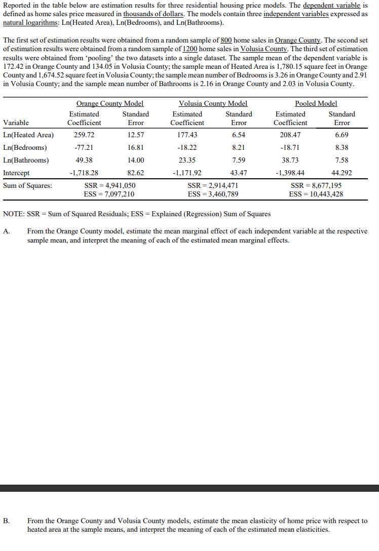
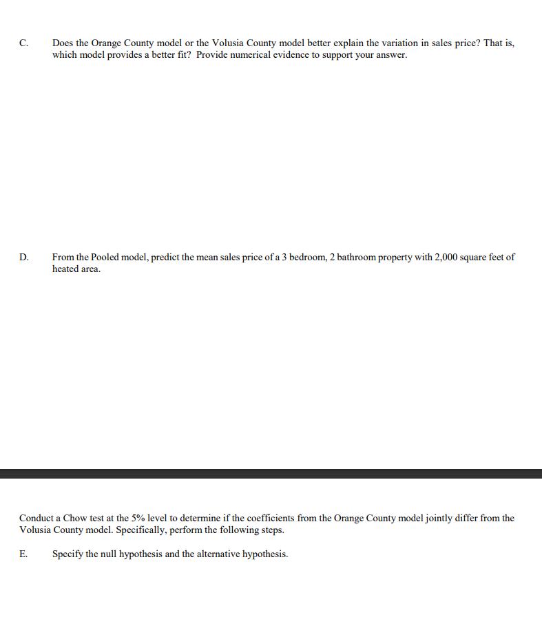
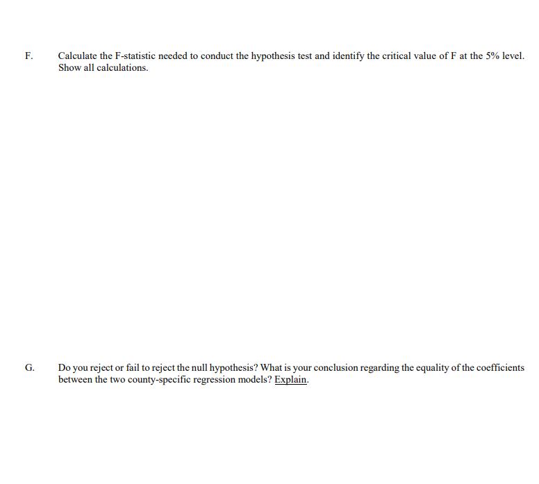
Reported in the table below are estimation results for three residential housing price models. The dependent variable is defined as home sales price measured in thousands of dollars. The models contain three independent variables expressed as natural logarithms: Ln(Heated Area), Ln(Bedrooms), and Ln(Bathrooms). The first set of estimation results were obtained from a random sample of 800 home sales in Orange County. The second set of estimation results were obtained from a random sample of 1200 home sales in Volusia County. The third set of estimation results were obtained from 'pooling' the two datasets into a single dataset. The sample mean of the dependent variable is 172.42 in Orange County and 134.05 in Volusia County; the sample mean of Heated Area is 1,780.15 square feet in Orange County and 1,674.52 square feet in Volusia County; the sample mean number of Bedrooms is 3.26 in Orange County and 2.91 in Volusia County; and the sample mean number of Bathrooms is 2.16 in Orange County and 2.03 in Volusia County. Variable Ln(Heated Area) Ln(Bedrooms) Ln(Bathrooms) Intercept Sum of Squares: A. Orange County Model B. Estimated Coefficient 259.72 -77.21 49.38 -1,718.28 Standard Error 12.57 16.81 14.00 82.62 SSR = 4,941,050 ESS=7,097,210 Volusia County Model Standard Error 6.54 8.21 7.59 43.47 Estimated Coefficient 177.43 -18.22 23.35 -1,171.92 SSR = 2,914,471 ESS = 3,460,789 Pooled Model Estimated Coefficient 208.47 -18.71 38.73 -1,398.44 Standard Error 6.69 8.38 7.58 44.292 NOTE: SSR = Sum of Squared Residuals; ESS = Explained (Regression) Sum of Squares From the Orange County model, estimate the mean marginal effect of each independent variable at the respective sample mean, and interpret the meaning of each of the estimated mean marginal effects. SSR = 8,677,195 ESS 10,443,428 From the Orange County and Volusia County models, estimate the mean elasticity of home price with respect to heated area at the sample means, and interpret the meaning of each of the estimated mean elasticities. C. D. Does the Orange County model or the Volusia County model better explain the variation in sales price? That is, which model provides a better fit? Provide numerical evidence to support your answer. From the Pooled model, predict the mean sales price of a 3 bedroom, 2 bathroom property with 2,000 square feet of heated area. Conduct a Chow test at the 5% level to determine if the coefficients from the Orange County model jointly differ from the Volusia County model. Specifically, perform the following steps. E. Specify the null hypothesis and the alternative hypothesis. F. G. Calculate the F-statistic needed to conduct the hypothesis test and identify the critical value of F at the 5% level. Show all calculations. Do you reject or fail to reject the null hypothesis? What is your conclusion regarding the equality of the coefficients between the two county-specific regression models? Explain.