resistivity data analysis
You should write and test the code for this exercise on your own machine and past it into the script window below when you want to submit it. Your code will then be assessed and marks and feedback given. You can change the code based on the feedback and resubmit as many times as you like.
Open the data file Matula.xlsx provided on Canvas. There are two columns, the first is temperature T in Kelvin, the second is resistivity p measured in an unknown unit for a certain metal. One would expect p to be given by:
P(T) = a + BT^5 (1)
Where a and b are constants.
We can plot a straight line graph by plotting p(T) on the y axis and T^5 on the x axis.
The purpose of this exercise is to calculate the values of a and B and plot graphs showing the fit. Use what has been covered in the first part of the lab to do this The steps involved are listed below. The mark for this assignment depends on successful completion of each step. Remember that you can check each step by running the script at any point. As this exercise is formative, the PGTAs are can assist you and give advice during the lab.
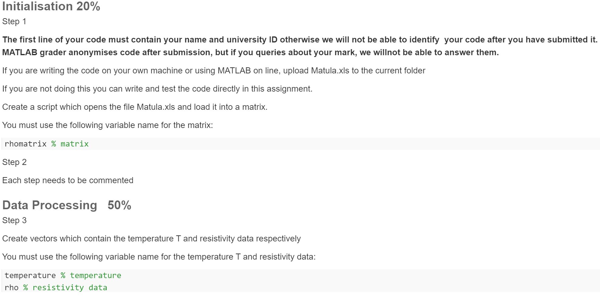
Initialisation 20%
Step 1
The first line of your code must contain your name and university ID otherwise we will not be able to identify your code after you have submitted it. MATLAB grader anonymises code after submission, but if you queries about your mark, we willnot be able to answer them.
If you are writing the code on your own machine or using MATLAB on line, upload Matula, xls to the current folder
If you are not doing this you can write and test the code directly in this assignment.
Create a script which opens the file Matula xis and load it into a matrix.
You must use the following variable name for the matrix:
rhomatrix matrix
Step 2
Each step needs to be commented
Data Processing 50%
Step 3
Create vectors which contain the temperature T and resistivity data respectively You must use the following variable name for the temperature T and resistivity data
temperature % temperature
rho % resistivity data
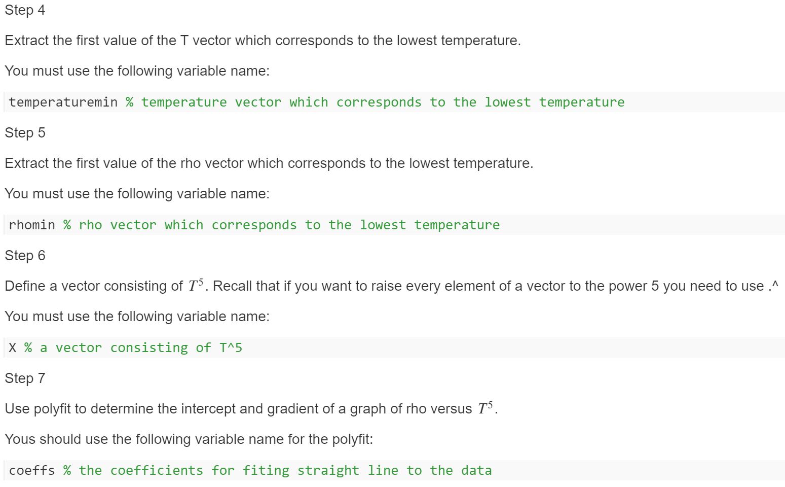
Step 4
Extract the first value of the T vector which corresponds to the lowest temperature.
You must use the following variable name:
temperaturemin % temperature vector which corresponds to the lowest temperature
Step 5
Extract the first value of the rho vector which corresponds to the lowest temperature.
You must use the following variable name:
rhomin % rho vector which corresponds to the lowest temperature
Step 6
Define a vector consisting of TS. Recall that if you want to raise every element of a vector to the power 5 you need to use.
You must use the following variable name:
X % a vector consisting of T 5
Step 7
Use polyfit to determine the intercept and gradient of a graph of rho versus 7*.
Yous should use the following variable name for the polyfit:
coeffs % the coefficients for fiting straight line to the data
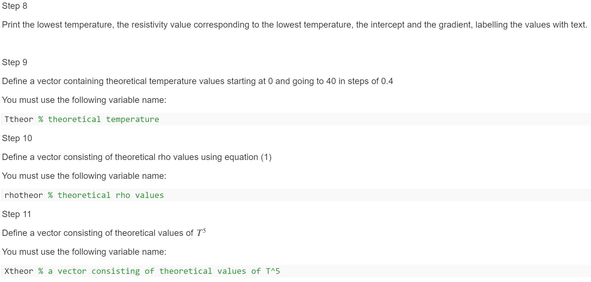
Step 8
Print the lowest temperature, the resistivity value corresponding to the lowest temperature, the intercept and the gradient, labelling the values with text.
Step 9
Define a vector containing theoretical temperature values starting at 0 and going to 40 in steps of 0.4
You must use the following variable name:
Ttheor % theoretical temperature
Step 10
Define a vector consisting of theoretical rho values using equation (1)
You must use the following variable name:
rhotheor % theoretical rho values
Step 11
Define a vector consisting of theoretical values of T
You must use the following variable name:
Xtheor % a vector consisting of theoretical values of TA5
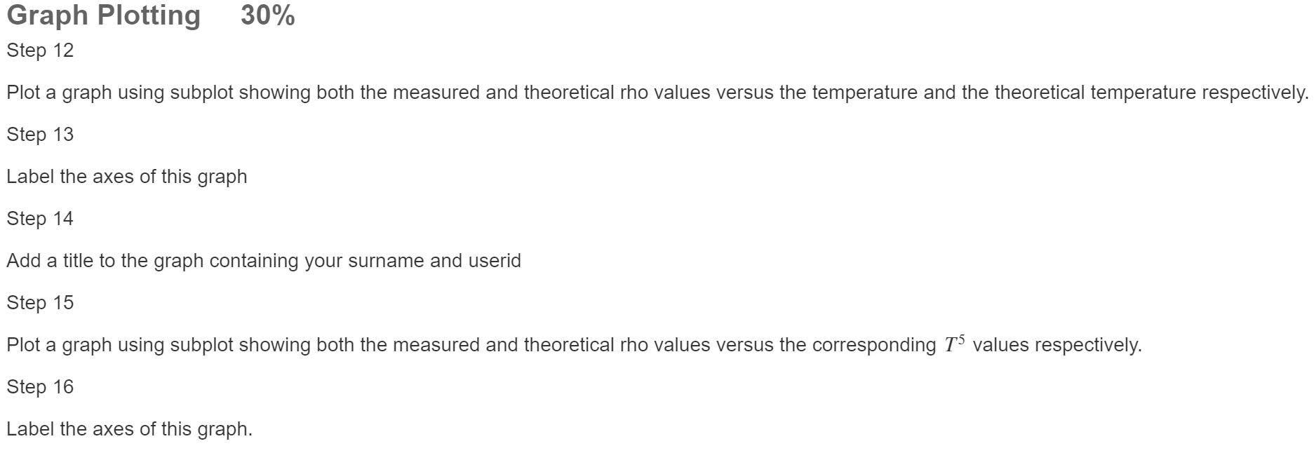
Graph Plotting
Step 12
30%
Plot a graph using subplot showing both the measured and theoretical rho values versus the temperature and the theoretical temperature respectively.
Step 13
Label the axes of this graph
Step 14
Add a title to the graph containing your surname and userid
Step 15
Plot a graph using subplot showing both the measured and theoretical rho values versus the corresponding T values respectively.
Step 16
Label the axes of this graph.


resistivity data analysis You should write and test the code for this exercise on your own machine and past it into the script window below when you want to submit it. Your code will then be assessed and marks and feedback given. You can change the code based on the feedback and resubmit as many times as you like. Open the data file Matula.xlsx provided on Canvas. There are two columns, the first is temperature T in Kelvin, the second is resistivity p measured in an unknown unit for a certain metal. One would expect p to be given by: P(T) = a + BT (1) Where a and are constants. We can plot a straight line graph by plotting P(T)on the y axis and is on the x axis. The purpose of this exercise is to calculate the values of a and B and plot graphs showing the fit. Use what has been covered in the first part of the lab to do this. The steps involved are listed below. The mark for this assignment depends on successful completion of each step. Remember that you can check each step by running the script at any point. As this exercise is formative, the PGTAs are can assist you and give advice during the lab. Initialisation 20% Step 1 The first line of your code must contain your name and university ID otherwise we will not be able to identify your code after you have submitted it. MATLAB grader anonymises code after submission, but if you queries about your mark, we willnot be able to answer them. If you are writing the code on your own machine or using MATLAB on line, upload Matula.xls to the current folder If you are not doing this you can write and test the code directly in this assignment. Create a script which opens the file Matula.xls and load it into a matrix. You must use the following variable name for the matrix: rhomatrix % matrix Step 2 Each step needs to be commented Data Processing 50% Step 3 Create vectors which contain the temperature T and resistivity data respectively You must use the following variable name for the temperature T and resistivity data: temperature % temperature rho % resistivity data Step 4 Extract the first value of the T vector which corresponds to the lowest temperature. You must use the following variable name: temperaturemin % temperature vector which corresponds to the lowest temperature Step 5 Extract the first value of the rho vector which corresponds to the lowest temperature. You must use the following variable name: rhomin % rho vector which corresponds to the lowest temperature Step 6 Define a vector consisting of T. Recall that if you want to raise every element of a vector to the power 5 you need to use .^ You must use the following variable name: X % a vector consisting of T^5 Step 7 Use polyfit to determine the intercept and gradient of a graph of rho versus TS. Yous should use the following variable name for the polyfit: coeffs % the coefficients for fiting straight line to the data Step 8 Print the lowest temperature, the resistivity value corresponding to the lowest temperature, the intercept and the gradient, labelling the values with text. Step 9 Define a vector containing theoretical temperature values starting at 0 and going to 40 in steps of 0.4 You must use the following variable name: Ttheor % theoretical temperature Step 10 Define a vector consisting of theoretical rho values using equation (1) You must use the following variable name: rhotheor % theoretical rho values Step 11 Define a vector consisting of theoretical values of T5 You must use the following variable name: Xtheor % a vector consisting of theoretical values of T^5 30% Graph Plotting Step 12 Plot a graph using subplot showing both the measured and theoretical rho values versus the temperature and the theoretical temperature respectively. Step 13 Label the axes of this graph Step 14 Add a title to the graph containing your surname and userid Step 15 Plot a graph using subplot showing both the measured and theoretical rho values versus the corresponding T) values respectively. Step 16 Label the axes of this graph. resistivity data analysis You should write and test the code for this exercise on your own machine and past it into the script window below when you want to submit it. Your code will then be assessed and marks and feedback given. You can change the code based on the feedback and resubmit as many times as you like. Open the data file Matula.xlsx provided on Canvas. There are two columns, the first is temperature T in Kelvin, the second is resistivity p measured in an unknown unit for a certain metal. One would expect p to be given by: P(T) = a + BT (1) Where a and are constants. We can plot a straight line graph by plotting P(T)on the y axis and is on the x axis. The purpose of this exercise is to calculate the values of a and B and plot graphs showing the fit. Use what has been covered in the first part of the lab to do this. The steps involved are listed below. The mark for this assignment depends on successful completion of each step. Remember that you can check each step by running the script at any point. As this exercise is formative, the PGTAs are can assist you and give advice during the lab. Initialisation 20% Step 1 The first line of your code must contain your name and university ID otherwise we will not be able to identify your code after you have submitted it. MATLAB grader anonymises code after submission, but if you queries about your mark, we willnot be able to answer them. If you are writing the code on your own machine or using MATLAB on line, upload Matula.xls to the current folder If you are not doing this you can write and test the code directly in this assignment. Create a script which opens the file Matula.xls and load it into a matrix. You must use the following variable name for the matrix: rhomatrix % matrix Step 2 Each step needs to be commented Data Processing 50% Step 3 Create vectors which contain the temperature T and resistivity data respectively You must use the following variable name for the temperature T and resistivity data: temperature % temperature rho % resistivity data Step 4 Extract the first value of the T vector which corresponds to the lowest temperature. You must use the following variable name: temperaturemin % temperature vector which corresponds to the lowest temperature Step 5 Extract the first value of the rho vector which corresponds to the lowest temperature. You must use the following variable name: rhomin % rho vector which corresponds to the lowest temperature Step 6 Define a vector consisting of T. Recall that if you want to raise every element of a vector to the power 5 you need to use .^ You must use the following variable name: X % a vector consisting of T^5 Step 7 Use polyfit to determine the intercept and gradient of a graph of rho versus TS. Yous should use the following variable name for the polyfit: coeffs % the coefficients for fiting straight line to the data Step 8 Print the lowest temperature, the resistivity value corresponding to the lowest temperature, the intercept and the gradient, labelling the values with text. Step 9 Define a vector containing theoretical temperature values starting at 0 and going to 40 in steps of 0.4 You must use the following variable name: Ttheor % theoretical temperature Step 10 Define a vector consisting of theoretical rho values using equation (1) You must use the following variable name: rhotheor % theoretical rho values Step 11 Define a vector consisting of theoretical values of T5 You must use the following variable name: Xtheor % a vector consisting of theoretical values of T^5 30% Graph Plotting Step 12 Plot a graph using subplot showing both the measured and theoretical rho values versus the temperature and the theoretical temperature respectively. Step 13 Label the axes of this graph Step 14 Add a title to the graph containing your surname and userid Step 15 Plot a graph using subplot showing both the measured and theoretical rho values versus the corresponding T) values respectively. Step 16 Label the axes of this graph

