RIGHT CLICK IMAGE AND OPEN IN NEW TAB TO MAKE BIGGER

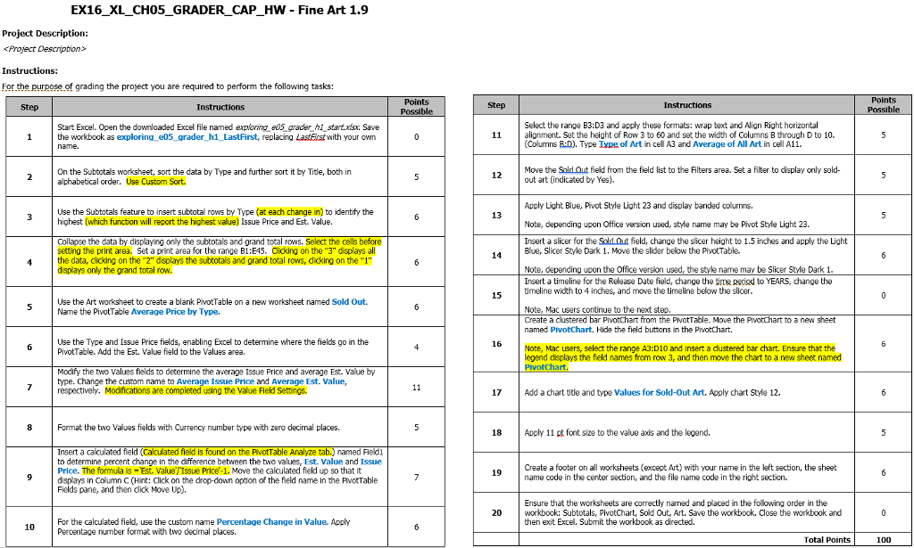
EX16_XL_CHO5_GRADER CAP_HW - Fine Art 1.9 Project Description: For the purpose of grading the project you are required to perform the following tasks: Select the range B3:D3 and apply these formats: wrap text and Align Right horizontal Columns B:D). Type Tyne of Art in cell A3 and Average of All Art in cell A11. Move the Sold Out field from the field list to the Filters area. Set a filter to display only sold- Start Excel. Open the downloaded Excel file named explonng e05 graderhi startxsx Save 1 the workbook as exploring e05_ grader h1 LastFirst, replacing LasEirst with your own 11 alignment. Set the height of Row 3 to 60 and set the width of Columns B through D to 10. On the Subtotals worksheet, sort the data by Type and further sort it by Tide, both in alphabetical order. Use Custom Sort. 12 out art (indicated by Yes). Apply Light Blue, Pivot Style Light 23 and display banded colunns. Note, depending upon Office version used, style name may be Pivot Style Light 23. Insert a slicer for the Sold Out field, change the slicer height to 1.5 inches and apply the Light Use the Subtotals feature to insert subtotal rows by Type (at each change in) to identify the highest (which function will report the highest value) Issue Price and Est. Value. Collapse the data by displaying only the subtotals and grand total rows setting the print area. Set a print area for the range B1:E45. Cicking on the "3" displays all Blue, Slicer Style Dark 1. Move the slider below the PivctTable. 14 4 the data, dicking on the "2" dsplays the subtotals and grand total rows, dicking on the "1" Note, depending upon the Office version used, the style name may be Slicer Style Dark 1 Insert a timeline for the Release Date field, change the tirme Reriad to YEARS, change the timeline width to 4 inches, and move the timeline below the slicer displays only the grand total row. 15 Ulse the Art worksheet to create a blank PivotTable on a new worksheet named Sold Out. Name the PivotTable Average Price by Type. Note, Mac users continue to the next step. Create a clustered bar Pivotchart from the PtvotTable. Move the Pivotchart to a new sheet named PivotChart. Hide the field buttons in the PivotChart. Use the Type and Issue Price fields, enabling Excel to determine where the fields go in the PivotTable. Add the Est. Value field to the Values area. Note, Mac users, select the range A3:D10 and insert a dlustered bar chart. Ensure that the legend displays the field names from row 3, and then move the chart to a new sheet named Modify the two Values fields to determine the average Issue Price and average Est. Value by type. Change the custom name to Average Issue Price and Average Est. Value, respectively. Modifications are completed using the value Fleld Settings. 17 Add a chart title and type Values for Sold-Out Art. Apply chart Style 12. Format the two Values fields with Currency number type with zero decimal places 18 Apply 11 ct font size to the value axis and the legend. is on the PiWotT lyze tab.) named Field1 nsert a to determine percent change in the difference between the two values, Est. Value and Issue Price. The formula is-Est. Value'Issue Price'-1. Move the calculated field up so that it displays in Column C (Hint: Click on the drop-down option of the field name In the PIVOtTable Fields pane, and then dlick Move Up). Create a footer on all worksheets (except Art) with your name in the left section, the sheet name code in the center section, and the file name code in the right section. 19 Ensure that the worksheets are correctly naned and placed in the following order in the 20 workbock: Subtotals, PivotChart, Sold Out, Art. Save the workbock, dose the workbook and For the calculated field, use the custom name Percentage Change in Value. Apply Percentage number format with two decimal places. hen exit Excel. Submit the workbook as directed. Total Points 100 EX16_XL_CHO5_GRADER CAP_HW - Fine Art 1.9 Project Description: For the purpose of grading the project you are required to perform the following tasks: Select the range B3:D3 and apply these formats: wrap text and Align Right horizontal Columns B:D). Type Tyne of Art in cell A3 and Average of All Art in cell A11. Move the Sold Out field from the field list to the Filters area. Set a filter to display only sold- Start Excel. Open the downloaded Excel file named explonng e05 graderhi startxsx Save 1 the workbook as exploring e05_ grader h1 LastFirst, replacing LasEirst with your own 11 alignment. Set the height of Row 3 to 60 and set the width of Columns B through D to 10. On the Subtotals worksheet, sort the data by Type and further sort it by Tide, both in alphabetical order. Use Custom Sort. 12 out art (indicated by Yes). Apply Light Blue, Pivot Style Light 23 and display banded colunns. Note, depending upon Office version used, style name may be Pivot Style Light 23. Insert a slicer for the Sold Out field, change the slicer height to 1.5 inches and apply the Light Use the Subtotals feature to insert subtotal rows by Type (at each change in) to identify the highest (which function will report the highest value) Issue Price and Est. Value. Collapse the data by displaying only the subtotals and grand total rows setting the print area. Set a print area for the range B1:E45. Cicking on the "3" displays all Blue, Slicer Style Dark 1. Move the slider below the PivctTable. 14 4 the data, dicking on the "2" dsplays the subtotals and grand total rows, dicking on the "1" Note, depending upon the Office version used, the style name may be Slicer Style Dark 1 Insert a timeline for the Release Date field, change the tirme Reriad to YEARS, change the timeline width to 4 inches, and move the timeline below the slicer displays only the grand total row. 15 Ulse the Art worksheet to create a blank PivotTable on a new worksheet named Sold Out. Name the PivotTable Average Price by Type. Note, Mac users continue to the next step. Create a clustered bar Pivotchart from the PtvotTable. Move the Pivotchart to a new sheet named PivotChart. Hide the field buttons in the PivotChart. Use the Type and Issue Price fields, enabling Excel to determine where the fields go in the PivotTable. Add the Est. Value field to the Values area. Note, Mac users, select the range A3:D10 and insert a dlustered bar chart. Ensure that the legend displays the field names from row 3, and then move the chart to a new sheet named Modify the two Values fields to determine the average Issue Price and average Est. Value by type. Change the custom name to Average Issue Price and Average Est. Value, respectively. Modifications are completed using the value Fleld Settings. 17 Add a chart title and type Values for Sold-Out Art. Apply chart Style 12. Format the two Values fields with Currency number type with zero decimal places 18 Apply 11 ct font size to the value axis and the legend. is on the PiWotT lyze tab.) named Field1 nsert a to determine percent change in the difference between the two values, Est. Value and Issue Price. The formula is-Est. Value'Issue Price'-1. Move the calculated field up so that it displays in Column C (Hint: Click on the drop-down option of the field name In the PIVOtTable Fields pane, and then dlick Move Up). Create a footer on all worksheets (except Art) with your name in the left section, the sheet name code in the center section, and the file name code in the right section. 19 Ensure that the worksheets are correctly naned and placed in the following order in the 20 workbock: Subtotals, PivotChart, Sold Out, Art. Save the workbock, dose the workbook and For the calculated field, use the custom name Percentage Change in Value. Apply Percentage number format with two decimal places. hen exit Excel. Submit the workbook as directed. Total Points 100