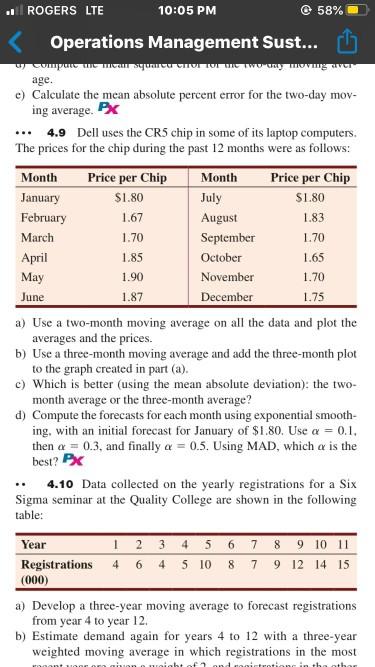
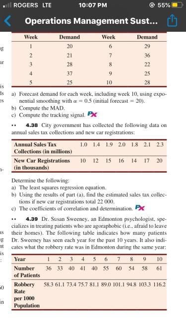
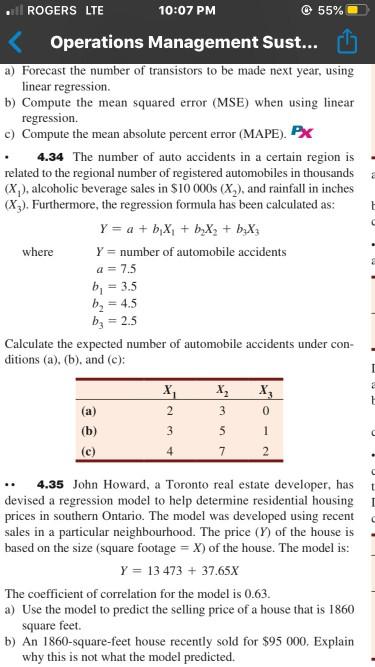
ROGERS LTE 10:05 PM 58% Operations Management Sust... age. c) Calculate the mean absolute percent error for the two-day mov- ing average. PX 4.9 Dell uses the CR5 chip in some of its laptop computers. The prices for the chip during the past 12 months were as follows: Month Price per Chip Month Price per Chip January $1.80 July SL.80 February 1.67 August 1.83 March 1.70 September 1.70 April 1.85 October 1.65 May 1.90 November 1.70 June 1.87 December 1.75 a) Use a two-month moving average on all the data and plot the averages and the prices. b) Use a three-month moving average and add the three-month plot to the graph created in part (a). c) Which is better (using the mean absolute deviation): the two- month average or the three-month average? d) Compute the forecasts for each month using exponential smooth- ing, with an initial forecast for January of $1.80. Use a = 0.1. then a = 0.3, and finally a = 0.5. Using MAD, which a is the best? 4.10 Data collected on the yearly registrations for a Six Sigma seminar at the Quality College are shown in the following table: Year 1 2 3 4 5 6 7 8 9 10 11 Registrations 4 6 4 5 10 8 7 9 12 14 15 (000) a) Develop a three-year moving average to forecast registrations from year 4 to year 12. b) Estimate demand again for years 4 to 12 with a three-year weighted moving average in which registrations in the most ROGERS LTE 10:07 PM 55% Operations Management Sust... Week 1 2 ar 8 4 is Ats es Demand Week Demand 20 6 29 21 7 36 3 28 22 37 9 25 5 25 10 28 a) Forecast demand for each week, including week 10. using expo- nential smoothing with a = 0.5 (initial forecast = 20). b) Compute the MAD c) Compute the tracking signal. PX 4.38 City government has collected the following data on annual sales tax collections and new car registrations: Annual Sales Tax 1.0 1.4 1.9 2.0 1.8 2.1 2.3 Collections (in millions) New Car Registrations 10 12 15 16 14 17 20 (in thousands) Determine the following: a) The least squares regression equation. b) Using the results of part (a), find the estimated sales tax collec- tions if new car registrations total 22 000. c) The coefficients of correlation and determination. PX 4.39 Dr. Susan Sweeney, an Edmonton psychologist, spe- cializes in treating patients who are agoraphobic (i.e., afraid to leave as their homes). The following table indicates how many patients & Dr. Sweeney has seen each year for the past 10 years. It also indi- mtcates what the robbery rate was in Edmonton during the same year Year 1 2 3 4 5 6 7 8 9 10 Number 36 33 40 41 40 55 60 54 58 61 of Patients 50 Robbery 58.3 61.1 73.4 75.7 81.1 89.0 101.1 94.8 103.3 116.2 Rate per 1000 Population is : in . ROGERS LTE 10:07 PM 0 55% 2 Operations Management Sust... a) Forecast the number of transistors to be made next year, using linear regression. b) Compute the mean squared error (MSE) when using linear regression c) Compute the mean absolute percent error (MAPE). PX 4.34 The number of auto accidents in a certain region is related to the regional number of registered automobiles in thousands (X), alcoholic beverage sales in S10 000s (X2), and rainfall in inches (X3). Furthermore, the regression formula has been calculated as: Y = a + b Xi + bxX, + bxX; where Y = number of automobile accidents a = 7.5 b, = 3.5 b = 4.5 by = 2.5 Calculate the expected number of automobile accidents under con- ditions (a), (b), and (c): X, (a) 2 3 0 (b) 3 5 1 7 2 1 4 4.35 John Howard, a Toronto real estate developer, has devised a regression model to help determine residential housing prices in southern Ontario. The model was developed using recent sales in a particular neighbourhood. The price (Y) of the house is based on the size (square footage = X) of the house. The model is: Y = 13 473 + 37.65X The coefficient of correlation for the model is 0.63. a) Use the model to predict the selling price of a house that is 1860 square feet b) An 1860-square-feet house recently sold for $95 000. Explain why this is not what the model predicted. ROGERS LTE 10:06 PM @ 56% Operations Management Sust... ... Usi fore tion mo Prot sho . exp! 9. C Tab dep The director of medical services predicted six years ago that demand in year I would be 41 surgeries. a) Use exponential smoothing, first with a smoothing constant of 0.6 and then with one of 0.9, to develop forecasts for years 2 through 6. b) Use a three-year moving average to forecast demand in years 4. 5. and 6. c) Use the trend projection method to forecast demand in years! through 6. d) With MAD as the criterion, which of the four forecasting meth- ods is best? 4.14 Following are two weekly forecasts made by two dif- ferent methods for the number of litres of gasoline, in thousands, demanded at a local gasoline station. Also shown are actual demand levels, in thousands of litres: Forecasts Week Method 1 Method 2 Actual Demand 1 0.90 0.80 0.70 2 1.05 1.20 1.00 3 0.95 0.90 1.00 4 1.20 1.11 1.00 What are the MAD and MSE for each method? 4.15 Refer to Solved Problem 4.1. Use a three-year mov- ing average to forecast the sales of Chevrolet Camaros in Alberta through 2016. What is the MAD? PX 4.16 Refer to Solved Problem 4.1. Using the trend projec- tion method, develop a forecast for the sales of Chevrolet Camaros in Alberta through 2016. What is the MAD? PX 4.17 Refer to Solved Problem 4.1. Using smoothing con- stants of 0.6 and 0.9, develop forecasts for the sales of Chevrolet Camaros. What effect did the smoothing constant have on the Mar ma Apr M Jul Au Se Oc Na De Jan Fel M. Ap ME . Jur 142 PART 1 Introduction to Operations Management a) Compute MAD and MAPE for management's technique. 4.28 ROGERS LTE 10:06 PM @ 57% Operations Management Sust... T 1 2 4 50 42 56 F 50 50 48 50 3 4 46 The first forecast, Fj, was derived by observing A, and setting F, equal to A. Subsequent forecasts were derived by exponential smoothing. Using the exponential smoothing method, find the forecast for time period 5. (Hint: You need first to find the smoothing constant, a.) 4.19 Income at the law firm Smith and Jones for the period February to July was as follows: Month February March April May June July Income 70.0 68.5 64.8 717 71.3 72.8 (in $000s) Use trend-adjusted exponential smoothing to forecast the law firm's August income. Assume that the initial forecast for February is $65 000 and the initial trend adjustment is 0. The smoothing con- stants selected are c = 0.1 and 8 = 0.2. PX 4.20 Resolve Problem 4.19 with a = 0.1 and 8 = 0.8. Using MSE, determine which smoothing constants provide a better forecast 4.21 Refer to the trend-adjusted exponential smoothing illustra- tion in Example 7. Using a = 0.2 and 3 = 0.4. we forecast sales for nine months, showing the detailed calculations for months 2 and 3. In Solved Problem 4.2, we continued the process for month 4. In this problem, show your calculations for months 5 and 6 for F, T, and FIT, PX 4.22 Refer to Problem 4.21. Complete the trend-adjusted exponential smoothing forecast computations for periods 7. 8. and 9. Confirm that your numbers for F, T, and FIT, match those in Table 4.2. PX 4.23 Sales of vegetable dehydrators at Bud Banis's discount department store in Gander over the past year are shown below. Management prepared a forecast using a combination of exponential . .. ROGERS LTE 10:06 PM @ 58% Operations Management Sust... best? PX 4.10 Data collected on the yearly registrations for a Six Sigma seminar at the Quality College are shown in the following table: Year 1 2 3 4 5 6 7 8 9 10 11 Registrations 4 6 4 5 10 8 7 9 12 14 15 (000) a) Develop a three-year moving average to forecast registrations from year 4 to year 12. b) Estimate demand again for years 4 to 12 with a three-year weighted moving average in which registrations in the most recent year are given a weight of 2, and registrations in the other two years are each given a weight of 1. c) Graph the original data and the two forecasts. Which of the two forecasting methods seems better? PX Chapter 4 Forecasting stant of forecast? Use MAD to determine which of the three smoothing m 4.10. stants (0.3.0.6, or 0.9) gives the most accurate forecast. PX 1 was .... 4.18 Consider the following actual (A) and forecast demand levels for a product: Time Period, Actual Demand, Forecast Deman Hemand T A F rant: 1 50 50 50 2 3 4 42 56 48 50 46 S