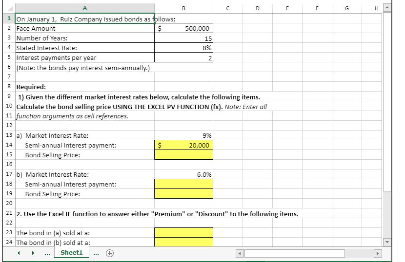
Ruiz Company issued bonds on January 1 and has provided the relevant information. The Controller has asked you to calculate the bond selling price given two different market interest rates using Excel’s Present Value functions. Use the information included in the Excel Simulation and the Excel functions described below to complete the task.

• Cell Reference: Allows you to refer to data from another cell in the worksheet. From the Excel Simulation below, if in a blank cell, “=B2” was entered, the formula would output the result from cell B2, or $500,000 in this example.
• Basic Math functions: Allows you to use the basic math symbols to perform mathematical functions. You can use the following keys: + (plus sign to add), - (minus sign to subtract), * (asterisk sign to multiply), and / (forward slash to divide). From the Excel Simulation below, if in a blank cell “=B3+B5” was entered, the formula would add the values from those cells and output the result, or 31 in this example. If using the other math symbols the result would output an appropriate answer for its function.
• PV Function: Allows you to perform the mathematical present value calculation of a value. The syntax of the PV function is “=PV(rate,nper,pmt,[fv],[type])” and results in the total amount that a series of future payments is worth now also known as the present value. The rate argument is the interest rate per period. The nper argument is the total number of payment periods. The pmt argument is the payment made each period that does not change over the life of the investment and this argument must be included if the [fv] argument is not included. The [fv] argument is the future value, or the cash basis to attain after the last payment is made and this argument must be included if the pmt argument is omitted. The [type] argument is a logical value of 0 or 1, which indicates when the payments are due where 1 is the payment at the beginning of the period and 0, is the payment at the end of the period. Both the [fv] and [type] values are optional arguments to have the formula work, which is why they are surrounded by brackets in the syntax, however, these values would not be entered with brackets in the actual function. For the purposes of this Excel Simulation, please include the [pmt] and [fv] arguments, but leave out the [type] argument from the function. Also, the [pmt] and [fv] arguments should be entered as negative values.
• IF function: Allows you to test a condition and return a specific value is the result is true and different value if the result is false. The syntax of the IF function is “=IF(test_condition,value_if_true,value_if_false)” and specific considerations need to be made when using this function. The test_condition argument is an evaluation of the status of a cell, such as if the value of a cell is greater than, less than, or equal to another number or cell. The value_if_true and value_if_false arguments will return any specific result for each option, such as another cell reference, a value, or text. Throughout the entire equation, if text is being used in the test_condition, value_if_true, or value_if_false arguments then the text itself should be entered in quotations so that Excel will recognize the text as a “string of text” instead of another function. From the Excel Simulation below, if in a blank cell “=IF(B2>250000,”Cash is great”,”Cash is bad”) was entered, the formula would output the result of the value_if_true since the test_condition would be result as true, or in this case the text “Cash is great”. Excel processes the IF function by separating it out into separate parts. First the test_condition – Excel thinks, find cell B2 and determine if the value is greater than 250000. Once Excel determines if the result of that test_condition is TRUE or FALSE, it will return the value_if_true or value_if_false.

A B D E 1 On January 1, Ruiz Company issued bonds as follows: 2 Face Amount $ 3 Number of Years: 4 Stated Interest Rate: 8% 5 Interest payments per year 2 6 (Note: the bonds pay interest semi-annually.) 7 8 Required: 91) Given the different market interest rates below, calculate the following items. 10 Calculate the bond selling price USING THE EXCEL PV FUNCTION (fx). Note: Enter all 11 function arguments as cell references. 12 13 a) Market Interest Rate: 9% $ 20,000 14 Semi-annual interest payment: 15 Bond Selling Price: 16 17 b) Market Interest Rate: 6.0% 18 Semi-annual interest payment: 19 Bond Selling Price: 20 21 2. Use the Excel IF function to answer either "Premium" or "Discount" to the following items. 22 23 The bond in (a) sold at a: 24 The bond in (b) sold at a: Sheet1 4 ... 567 500,000 15 C F G H [] 4