Scenario: Balky Modi, the CFO for the firm PSUWC Designer Shoes Company, LLC, woke up with a start at 4:00 am on 4/24/2023, due to the phone ringing. It was the firms senior financial analyst, vacationing in Europe, calling with bad news. Balky was supposed to present the project evaluation, at the end of the week, for the Board's proposal that they invest in new equipment which would enable them to add a new product line. Currently PSUWC has four successful products and they are considering selling a new Designer Shoes line. The staff of financial analysts had been working hard over the last few weeks collecting data and had prepared a model creating a financial forecast about the proposed project's viability. Disaster had struck on the night of 4/23/2023 wherein malware all but wiped out the work of the analysts. Balky needed to prepare a financial analysis of the project to present the Board with recommendations. All the staff had already left for their annual vacation and Balky was working alone. Balky quickly reached the office and managed to salvage what was left of the excel spreadsheet prepared for the presentation. What follows is some basic information that Balky knew and was able to retrieve about the project. PSUWC's existing plant has excess capacity, in a fully depreciated building, to install and run the new equipment to produce the new Designer Shoes line. Due to relatively rapid advances in technology, the project was expected to be discontinued in four years. The new Designer Shoes was expected to sell for $ 117 per unit and had projected sales of 4100 units in the first year, with a projected (Most-Likely scenario) 20.0 % growth rate per year for subsequent years. A total investment of $ 772,000 for new equipment was required. The equipment had fixed maintenance contracts of $ 237,103 per year with a salvage value of $ 132,485 and variable costs were 5 % of revenues. Balky also needed to consider both the Best-Case and Worst-Case scenarios in the analysis with growth rates of 30.00 % and 2.00 % respectively.

The new equipment would be depreciated to zero using straight line depreciation. The new project required an increase in working capital of $ 207,890 and $ 20,789 of this increase would be offset with accounts payable. PSUWC currently has 896000 shares of stock outstanding at a current price of $ 85.00. Even though the company has outstanding stock, it is not publicly traded and therefore there is no publicly available financial information. However, after analysis management believes that its equity beta is 0.91.

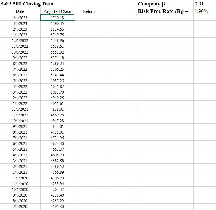
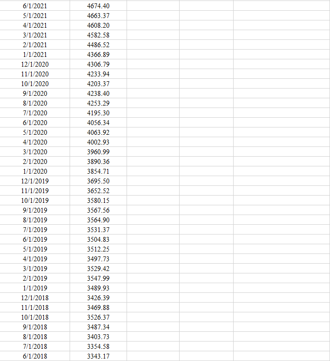
The company also has 77000 bonds outstanding, with a current price of $ 1,045.00. The bonds pay interest semi-annually at a coupon rate of 4.20 %. The bonds have a par value of $1,000 and will mature in 7 years. The average corporate tax rate was 33 %. Management believes the S&P 500 is a reasonable proxy for the market portfolio. Therefore, the cost of equity is calculated using the company's equity beta and the market risk premium based on the S&P 500 annual expected rate of return - Balky would calculate the monthly expected market return using 5 years of past monthly price data available in the worksheet Marketdata. This would then be multiplied by 12 to estimate the annual expected rate. Balky remembered that if the expected rate of return for the market was too low, too high, or negative, a forward looking rate of an historical average of about 9.5% would have to be used, as the calculated value for the current 5-year period may not be representative of the future. Balky would consider a E(Rm) between 8-12% acceptable. Balky would calculate the market risk premium: E(Rm) - Rf from the previous calculations using the risk-free rate data available in the worksheet Marketdata. Balky noted that the risk-free rate was on an annual basis. Balky needed to calculate the rate at which the project would have to be discounted to calculate the Net Present Value (NPV) of the proposed project based on the decision of raising capital and the current capital market environment. This discount rate, the WACC, would obviously influence the NPV and could affect the decision of whether to accept or reject the project. Thankfully, all the information needed to calculate this was available. Balky needed to clearly show all the calculations and sources for all parameter estimates used in the calculation of the WACC (and ultimately the NPV). Gathering all the available information, Balky got a large cup of extra strong coffee and sat down to work on the development of the Capital Budgeting project model. The correct recommendation to the board was critical to the future growth of the firm! Balky appreciated the detailed step by step instructions on the Worksheet 0.Case Instructions - Luckily they were still available!!.

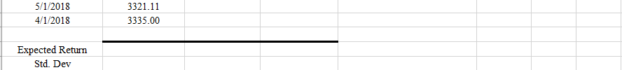
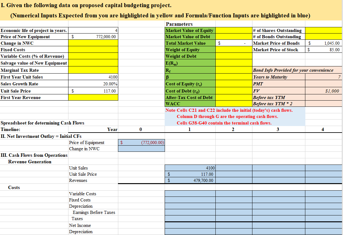
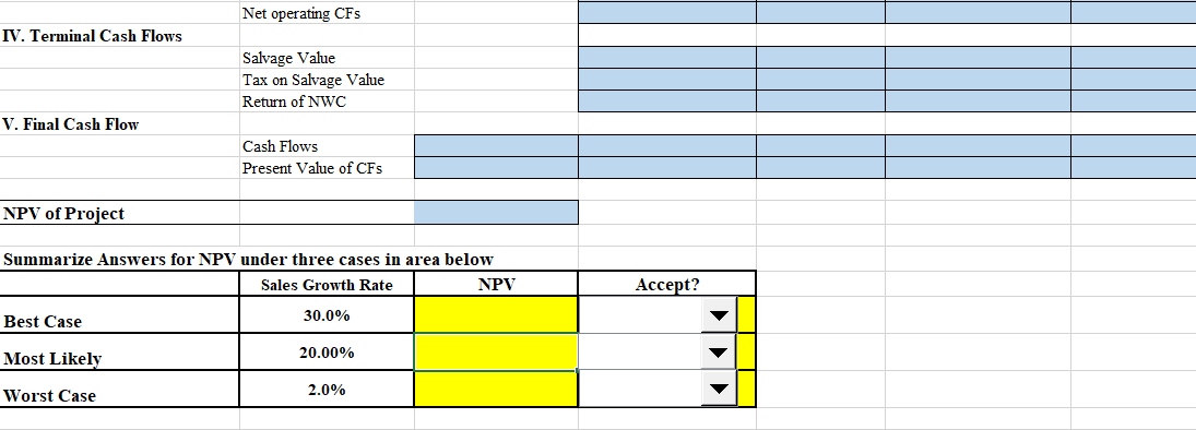
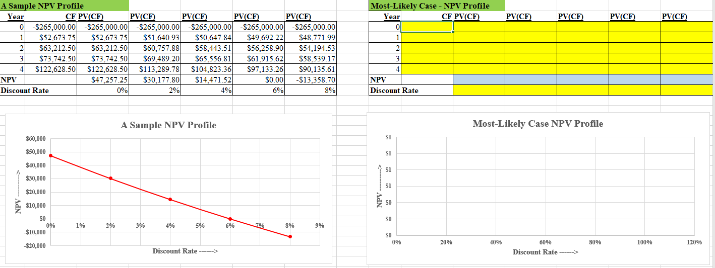
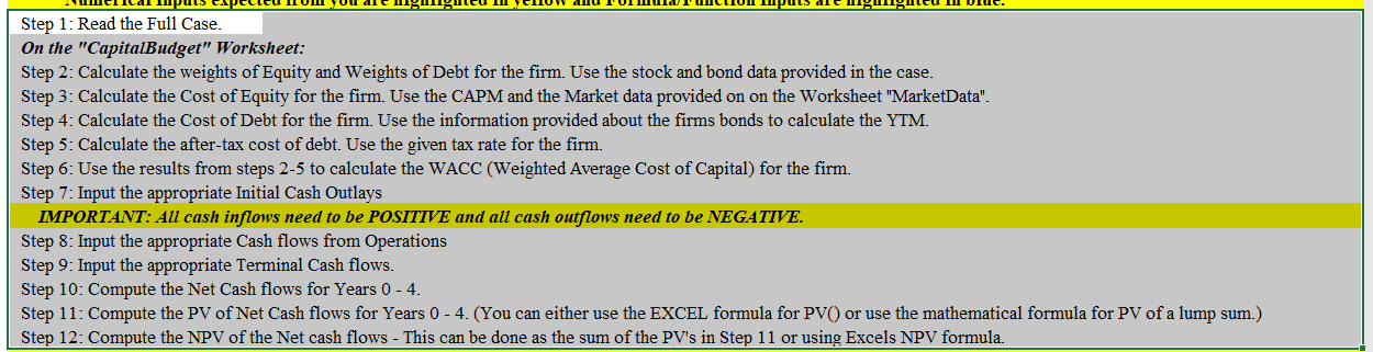
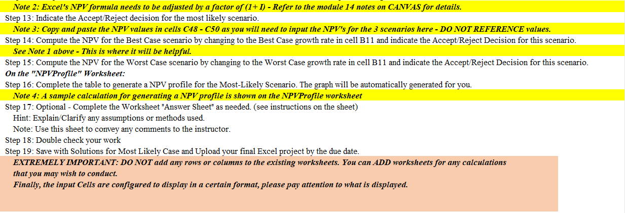
Note 1: Please use appropriate Cell referencing in Excel so that your numerical values update when you change any input(s). This will be helpful when you analyze the Best and Worst Case growth rate scenarios. Numerical Inputs expected from you are highlighted in yellow and Formula/Function Inputs are highlighted in blue. Step 1: Read the Full Case. On the "CapitalBudget" Worksheet: Step 2: Calculate the weights of Equity and Weights of Debt for the firm. Use the stock and bond data provided in the case. Step 3: Calculate the Cost of Equity for the firm. Use the CAPM and the Market data provided on on the Worksheet "MarketData". Step 4: Calculate the Cost of Debt for the firm. Use the information provided about the firms bonds to calculate the YTM. Step 5: Calculate the after-tax cost of debt. Use the given tax rate for the firm. Step 6: Use the results from steps 2-5 to calculate the WACC (Weighted Average Cost of Capital) for the firm. Step 7: Input the appropriate Initial Cash Outlays IMPORTANT: All cash inflows need to be POSITIVE and all cash outflows need to be NEGATIVE. Step 8: Input the appropriate Cash flows from Operations Step 9: Input the appropriate Terminal Cash flows. Step 10: Compute the Net Cash flows for Years 04. Step 11: Compute the PV of Net Cash flows for Years 0 - 4. (You can either use the EXCEL formula for PV() or use the mathematical formula for PV of a lump sum.) Step 12: Compute the NPV of the Net cash flows - This can be done as the sum of the PV's in Step 11 or using Excels NPV formula. Note 2: Excel's NPV formula needs to be adjusted by a factor of (1+I) Refer to the module 14 notes on CANVAS for details. Step 13: Indicate the Accept/Reject decision for the most likely scenario. Note 3: Copy and paste the NPV values in cells C48 - C50 as you will need to input the NPV's for the 3 scenarios here - DO NOT REFERENCE values. Step 14: Compute the NPV for the Best Case scenario by changing to the Best Case growth rate in cell B11 and indicate the Accept/Reject Decision for this scenario. See Note 1 above - This is where it will be helpful. Step 15: Compute the NPV for the Worst Case scenario by changing to the Worst Case growth rate in cell B11 and indicate the Accept/Reject Decision for this scenario. On the "NPVProfile" Worksheet: Step 16: Complete the table to generate a NPV profile for the Most-Likely Scenario. The graph will be automatically generated for you. Note 4: A sample calculation for generating a NPV profile is shown on the NPVProfile worksheet Step 17: Optional - Complete the Worksheet "Answer Sheet" as needed. (see instructions on the sheet) Hint: Explain/Clarify any assumptions or methods used. Note: Use this sheet to convey any comments to the instructor. Step 18: Double check your work Step 19: Save with Solutions for Most Likely Case and Upload your final Excel project by the due date. EXTREMELY IMPORTANT: DO NOT add any rows or columns to the existing worksheets. You can ADD worksheets for any calculations that you may wish to conduct. Finally, the input Cells are configured to display in a certain format, please pay attention to what is displayed. \begin{tabular}{|c|c|} \hline 6/1/2021 & 4674.40 \\ \hline 5/1/2021 & 4663.37 \\ \hline 4/1/2021 & 4608.20 \\ \hline 3/1/2021 & 4582.58 \\ \hline 2/1/2021 & 4486.52 \\ \hline 1/1/2021 & 4366.89 \\ \hline 12/1/2020 & 4306.79 \\ \hline 11/1/2020 & 4233.94 \\ \hline 10/1/2020 & 4203.37 \\ \hline 9/1/2020 & 4238.40 \\ \hline 8/1/2020 & 4253.29 \\ \hline 7/1/2020 & 4195.30 \\ \hline 6/1/2020 & 4056.34 \\ \hline 5/1/2020 & 4063.92 \\ \hline 4/1/2020 & 4002.93 \\ \hline 3/1/2020 & 3960.99 \\ \hline 2/1/2020 & 3890.36 \\ \hline 1/1/2020 & 3854.71 \\ \hline 12/1/2019 & 3695.50 \\ \hline 11/1/2019 & 3652.52 \\ \hline 10/1/2019 & 3580.15 \\ \hline 9/1/2019 & 3567.56 \\ \hline 8/1/2019 & 3564.90 \\ \hline 7/1/2019 & 3531.37 \\ \hline 6/1/2019 & 3504.83 \\ \hline 5/1/2019 & 3512.25 \\ \hline 4/1/2019 & 3497.73 \\ \hline 3/1/2019 & 3529.42 \\ \hline 2/1/2019 & 3547.99 \\ \hline 1/1/2019 & 3489.93 \\ \hline 12/1/2018 & 3426.39 \\ \hline 11/1/2018 & 3469.88 \\ \hline 10/1/2018 & 3526.37 \\ \hline 9/1/2018 & 3487.34 \\ \hline 8/1/2018 & 3403.73 \\ \hline 7/1/2018 & 3354.58 \\ \hline 6/1/2018 & 3343.17 \\ \hline \end{tabular} \begin{tabular}{|l|l|} \hline 5/1/2018 & 3321.11 \\ \hline 4/1/2018 & 3335.00 \\ \hline \end{tabular} Expected Return Std. Dev Given the following data on proposed capital budgeting project. NPV of Project Summarize Answers for NPV under three cases in area below \begin{tabular}{|l|c|c|c|} \hline & Sales Growth Rate & NPV & Accept? \\ \hline Best Case & 30.0% & & \\ \hline Most Likely & 20.00% & & \\ \hline Worst Case & 2.0% & & \\ \hline \end{tabular} \begin{tabular}{|r|r|r|r|r|r|r|} \hline A Sample NPV Profile \\ \hline \multicolumn{1}{|l|}{ Year } & CF & PV(CF) & \multicolumn{1}{l|}{ PV(CF) } & \multicolumn{1}{l|}{ PV(CF) } & \multicolumn{1}{l|}{ PV(CF) } & \multicolumn{1}{l|}{ PV(CF) } \\ \hline 0 & $265,000.00 & $265,000.00 & $265,000.00 & $265,000.00 & $265,000.00 & $265,000.00 \\ \hline 1 & $52,673.75 & $52,673.75 & $51,640.93 & $50,647.84 & $49,692.22 & $48,771.99 \\ \hline 2 & $63,212.50 & $63,212.50 & $60,757.88 & $58,443.51 & $56,258.90 & $54,194.53 \\ \hline 3 & $73,742.50 & $73,742.50 & $69,489.20 & $65,556.81 & $61,915.62 & $58,539.17 \\ \hline 4 & $122,628.50 & $122,628.50 & $113,289.78 & $104,823.36 & $97,133.26 & $90,135.61 \\ \hline NPV & & $47,257.25 & $30,177.80 & $14,471.52 & $0.00 & $13,358.70 \\ \hline Discount Rate & 0% & 2% & 4% & 6% & 8% \\ \hline \end{tabular} Most-Likely Case - NPV Profile Most-Likely Case NPV Profile Note 1: Please use appropriate Cell referencing in Excel so that your numerical values update when you change any input(s). This will be helpful when you analyze the Best and Worst Case growth rate scenarios. Numerical Inputs expected from you are highlighted in yellow and Formula/Function Inputs are highlighted in blue. Step 1: Read the Full Case. On the "CapitalBudget" Worksheet: Step 2: Calculate the weights of Equity and Weights of Debt for the firm. Use the stock and bond data provided in the case. Step 3: Calculate the Cost of Equity for the firm. Use the CAPM and the Market data provided on on the Worksheet "MarketData". Step 4: Calculate the Cost of Debt for the firm. Use the information provided about the firms bonds to calculate the YTM. Step 5: Calculate the after-tax cost of debt. Use the given tax rate for the firm. Step 6: Use the results from steps 2-5 to calculate the WACC (Weighted Average Cost of Capital) for the firm. Step 7: Input the appropriate Initial Cash Outlays IMPORTANT: All cash inflows need to be POSITIVE and all cash outflows need to be NEGATIVE. Step 8: Input the appropriate Cash flows from Operations Step 9: Input the appropriate Terminal Cash flows. Step 10: Compute the Net Cash flows for Years 04. Step 11: Compute the PV of Net Cash flows for Years 0 - 4. (You can either use the EXCEL formula for PV() or use the mathematical formula for PV of a lump sum.) Step 12: Compute the NPV of the Net cash flows - This can be done as the sum of the PV's in Step 11 or using Excels NPV formula. Note 2: Excel's NPV formula needs to be adjusted by a factor of (1+I) Refer to the module 14 notes on CANVAS for details. Step 13: Indicate the Accept/Reject decision for the most likely scenario. Note 3: Copy and paste the NPV values in cells C48 - C50 as you will need to input the NPV's for the 3 scenarios here - DO NOT REFERENCE values. Step 14: Compute the NPV for the Best Case scenario by changing to the Best Case growth rate in cell B11 and indicate the Accept/Reject Decision for this scenario. See Note 1 above - This is where it will be helpful. Step 15: Compute the NPV for the Worst Case scenario by changing to the Worst Case growth rate in cell B11 and indicate the Accept/Reject Decision for this scenario. On the "NPVProfile" Worksheet: Step 16: Complete the table to generate a NPV profile for the Most-Likely Scenario. The graph will be automatically generated for you. Note 4: A sample calculation for generating a NPV profile is shown on the NPVProfile worksheet Step 17: Optional - Complete the Worksheet "Answer Sheet" as needed. (see instructions on the sheet) Hint: Explain/Clarify any assumptions or methods used. Note: Use this sheet to convey any comments to the instructor. Step 18: Double check your work Step 19: Save with Solutions for Most Likely Case and Upload your final Excel project by the due date. EXTREMELY IMPORTANT: DO NOT add any rows or columns to the existing worksheets. You can ADD worksheets for any calculations that you may wish to conduct. Finally, the input Cells are configured to display in a certain format, please pay attention to what is displayed. \begin{tabular}{|c|c|} \hline 6/1/2021 & 4674.40 \\ \hline 5/1/2021 & 4663.37 \\ \hline 4/1/2021 & 4608.20 \\ \hline 3/1/2021 & 4582.58 \\ \hline 2/1/2021 & 4486.52 \\ \hline 1/1/2021 & 4366.89 \\ \hline 12/1/2020 & 4306.79 \\ \hline 11/1/2020 & 4233.94 \\ \hline 10/1/2020 & 4203.37 \\ \hline 9/1/2020 & 4238.40 \\ \hline 8/1/2020 & 4253.29 \\ \hline 7/1/2020 & 4195.30 \\ \hline 6/1/2020 & 4056.34 \\ \hline 5/1/2020 & 4063.92 \\ \hline 4/1/2020 & 4002.93 \\ \hline 3/1/2020 & 3960.99 \\ \hline 2/1/2020 & 3890.36 \\ \hline 1/1/2020 & 3854.71 \\ \hline 12/1/2019 & 3695.50 \\ \hline 11/1/2019 & 3652.52 \\ \hline 10/1/2019 & 3580.15 \\ \hline 9/1/2019 & 3567.56 \\ \hline 8/1/2019 & 3564.90 \\ \hline 7/1/2019 & 3531.37 \\ \hline 6/1/2019 & 3504.83 \\ \hline 5/1/2019 & 3512.25 \\ \hline 4/1/2019 & 3497.73 \\ \hline 3/1/2019 & 3529.42 \\ \hline 2/1/2019 & 3547.99 \\ \hline 1/1/2019 & 3489.93 \\ \hline 12/1/2018 & 3426.39 \\ \hline 11/1/2018 & 3469.88 \\ \hline 10/1/2018 & 3526.37 \\ \hline 9/1/2018 & 3487.34 \\ \hline 8/1/2018 & 3403.73 \\ \hline 7/1/2018 & 3354.58 \\ \hline 6/1/2018 & 3343.17 \\ \hline \end{tabular} \begin{tabular}{|l|l|} \hline 5/1/2018 & 3321.11 \\ \hline 4/1/2018 & 3335.00 \\ \hline \end{tabular} Expected Return Std. Dev Given the following data on proposed capital budgeting project. NPV of Project Summarize Answers for NPV under three cases in area below \begin{tabular}{|l|c|c|c|} \hline & Sales Growth Rate & NPV & Accept? \\ \hline Best Case & 30.0% & & \\ \hline Most Likely & 20.00% & & \\ \hline Worst Case & 2.0% & & \\ \hline \end{tabular} \begin{tabular}{|r|r|r|r|r|r|r|} \hline A Sample NPV Profile \\ \hline \multicolumn{1}{|l|}{ Year } & CF & PV(CF) & \multicolumn{1}{l|}{ PV(CF) } & \multicolumn{1}{l|}{ PV(CF) } & \multicolumn{1}{l|}{ PV(CF) } & \multicolumn{1}{l|}{ PV(CF) } \\ \hline 0 & $265,000.00 & $265,000.00 & $265,000.00 & $265,000.00 & $265,000.00 & $265,000.00 \\ \hline 1 & $52,673.75 & $52,673.75 & $51,640.93 & $50,647.84 & $49,692.22 & $48,771.99 \\ \hline 2 & $63,212.50 & $63,212.50 & $60,757.88 & $58,443.51 & $56,258.90 & $54,194.53 \\ \hline 3 & $73,742.50 & $73,742.50 & $69,489.20 & $65,556.81 & $61,915.62 & $58,539.17 \\ \hline 4 & $122,628.50 & $122,628.50 & $113,289.78 & $104,823.36 & $97,133.26 & $90,135.61 \\ \hline NPV & & $47,257.25 & $30,177.80 & $14,471.52 & $0.00 & $13,358.70 \\ \hline Discount Rate & 0% & 2% & 4% & 6% & 8% \\ \hline \end{tabular} Most-Likely Case - NPV Profile Most-Likely Case NPV Profile