Section 10.4 for more information: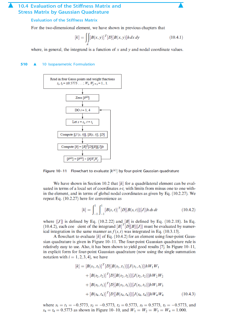

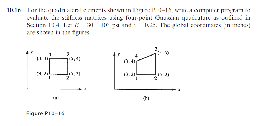
Evaluation of the Stiffness Matrix and Stress Matrix by Gaussian Quadrature Evaluation of the Stiffness Matrix For the two-dimensional element, we have shown in previous chapters that where, in general, the integrand is a function of x and y and nodal coordinate values. Isoparametric Formulation We have shown in Section 10.2 that [k] for a quadrilateral element can be evaluated in terms of a local set of coordinates s-t, with limits from minus one to one within the element, and in terms of global nodal coordinates as given by Eq. (10.2.27). We repeat Eq. (10.2.27) here for convenience as where |[J]| is defined by Eq. (10.2.22) and [B] is defined by Eq. (10.2.18). In Eq (10.4.2), each coefficient of the integrand [B]^T [D][B]|[J]| must be evaluated by numerical integration in the same manner as f (s, t) was integrated in Eq. (10.3.13) A flowchart to evaluate k of Eq. (10.4.2) for an element using four-point Gaussian quadrature is given in Figure 10-11 The four-point Gaussian quadrature rule is relatively easy to use. Also, it has been shown to yield good results [7]. In Figure 10-11 in explicit form for four-point Gaussian quadrature (now using the single summation notation with i 2, 3, 4), we have where s_1 = t_1 = -0.5773, s_2 = -0.5773, t_2 = 0.5773, s_3 = 0.5773, t_3 = 0.5773, and s_4 = 0.5773 as shown in Figure 10-10, and W_1 = W_2 = W_3 = W_4 = 1.000. For the quadrilateral elements shown in Figure P10-16, write a computer program to evaluate the stiffness matrices using four-point Gaussian quadrature as outlined in Section 10.4. Let E = 30 10^6 psi and v = 0.25. The global coordinates (in inches) are shown in the figures. Evaluation of the Stiffness Matrix and Stress Matrix by Gaussian Quadrature Evaluation of the Stiffness Matrix For the two-dimensional element, we have shown in previous chapters that where, in general, the integrand is a function of x and y and nodal coordinate values. Isoparametric Formulation We have shown in Section 10.2 that [k] for a quadrilateral element can be evaluated in terms of a local set of coordinates s-t, with limits from minus one to one within the element, and in terms of global nodal coordinates as given by Eq. (10.2.27). We repeat Eq. (10.2.27) here for convenience as where |[J]| is defined by Eq. (10.2.22) and [B] is defined by Eq. (10.2.18). In Eq (10.4.2), each coefficient of the integrand [B]^T [D][B]|[J]| must be evaluated by numerical integration in the same manner as f (s, t) was integrated in Eq. (10.3.13) A flowchart to evaluate k of Eq. (10.4.2) for an element using four-point Gaussian quadrature is given in Figure 10-11 The four-point Gaussian quadrature rule is relatively easy to use. Also, it has been shown to yield good results [7]. In Figure 10-11 in explicit form for four-point Gaussian quadrature (now using the single summation notation with i 2, 3, 4), we have where s_1 = t_1 = -0.5773, s_2 = -0.5773, t_2 = 0.5773, s_3 = 0.5773, t_3 = 0.5773, and s_4 = 0.5773 as shown in Figure 10-10, and W_1 = W_2 = W_3 = W_4 = 1.000. For the quadrilateral elements shown in Figure P10-16, write a computer program to evaluate the stiffness matrices using four-point Gaussian quadrature as outlined in Section 10.4. Let E = 30 10^6 psi and v = 0.25. The global coordinates (in inches) are shown in the figures