Section 9.1 Reading Assignment: Solutions, Slope Fields, and Euler's Method

Answer Only Exercise 1, 2, and 3 by using a screenshot provided Calculus Pearson textbook. Make sure you read these three questions very carefully and see on what it is asking for and what is really about.

References: Thomas' Calculus: Early Transcendentals | Calculus | Calculus | Mathematics | Store | Pearson+

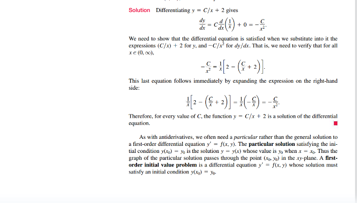
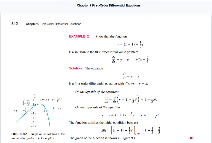
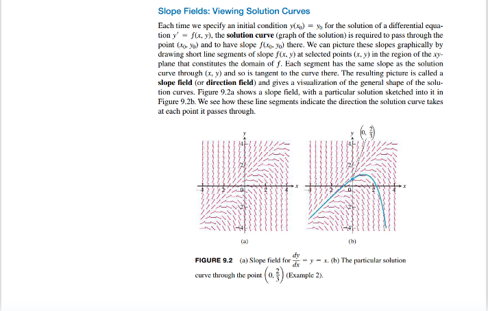
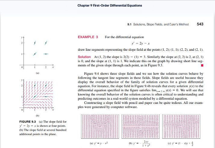
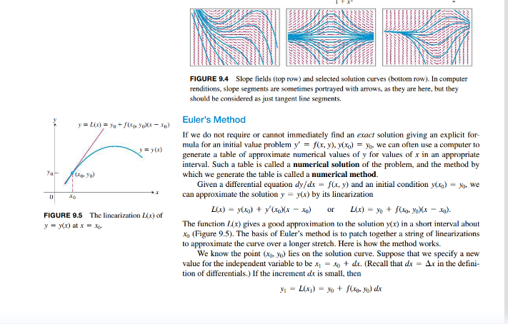
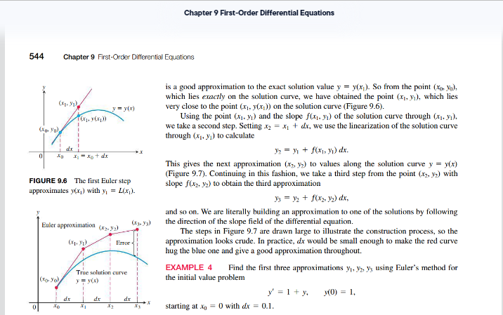
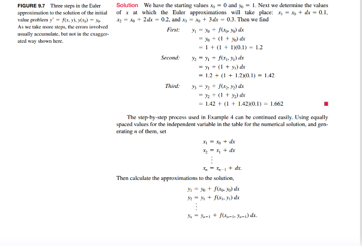
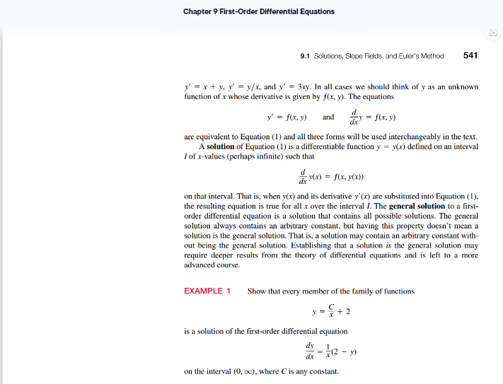
Section 9.1 Reading Assignment: Solutions, Slope Fields, and Euler's Method Instructions. Read through this assignment and complete the three exercises below by reading the appropriate passages of the textbook. We will be introducing differential equations here, which are equations that involve a function and its derivatives and the solution to a differential equation is a function. We will consider only rstorder differential equations in this class, which means the differential equations only contains the function y and its first derivative 2: or 3;\" (depending on which notation is being used). Exercise 1. Read Example 1 (p. 541) and Example 2 (p. 542). Explain how to verify a function or family of functions is a solution of a differential equation. Verifying solutions is just like checking your answers in algebra, except it involves some calculus. It's a good idea to verify your solutions when we solve differential equations later on. This is a useful skill to develop in the same way that checking answers in algebra can be useful. As Example 1 shows, the solution to a differential equation is actually a family of curves with an unknown constant C involved. This C is the same one we have when ta king indefinite integrals, though it will often get shuffled into the expression as we will explore later. Exercise 2. Read the subsection "Slope Fields: Viewing Solution Curves\" (p. 542 543). Explain how Example 3 (p. 543) and Figure 9.3 (margin of p. 543) shows how a slope field can be drawn. We will typically ayoicl drawing slope fields by hand, but it's useful to understand how to do so and how the slope field illustrates things about the differential equation. Exercise 3. Read the introduction to the subsection Euler's Method (p. 543 544}. Explain how linearization is used in the formula for Euler's method. Euler's method is an example of a numerical method which is used to approximate values when we can't find exact values. Chapter 9 First-Order Differential Equations 9.1 Solutions, Slope Fields, and Euler's Method 541 y' = x + y, y' = y/x, and y' = 3xy. In all cases we should think of y as an unknown function of x whose derivative is given by f(x, y). The equations y' = f(x, y) and Ly = f(x, y) are equivalent to Equation (1) and all three forms will be used interchangeably in the text. A solution of Equation (1) is a differentiable function y = >(x) defined on an interval / of x-values (perhaps infinite) such that Ly(x) = f(x yx) on that interval. That is, when y(x) and its derivative y'(x) are substituted into Equation (1), the resulting equation is true for all x over the interval /. The general solution to a first- order differential equation is a solution that contains all possible solutions. The general solution always contains an arbitrary constant, but having this property doesn't mean a solution is the general solution. That is, a solution may contain an arbitrary constant with- out being the general solution. Establishing that a solution is the general solution may require deeper results from the theory of differential equations and is left to a more advanced course. EXAMPLE 1 Show that every member of the family of functions C +2 is a solution of the first-order differential equation dx = (2 - y) on the interval (0, co). where C is any constant.Solution Differentiating y = C/x + 2 gives dy dx +0 =- We need to show that the differential equation is satisfied when we substitute into it the expressions (C/x) + 2 for y. and -C/x for dy/ dx. That is, we need to verify that for all X E (0, 00). This last equation follows immediately by expanding the expression on the right-hand side: */2 - (8 + 2 ) ] - 4( - 8 ) - -5 Therefore, for every value of C, the function y = C/x + 2 is a solution of the differential equation. As with antiderivatives, we often need a particular rather than the general solution to a first-order differential equation y' = f(x, y). The particular solution satisfying the ini- tial condition y(x ) = > is the solution y = y(x) whose value is yo when x = 1. Thus the graph of the particular solution passes through the point (xo. )) in the xy-plane. A first- order initial value problem is a differential equation y' = f(x, y) whose solution must satisfy an initial condition y(x) = Yo-Chapter 9 First-Order Differential Equations 542 Chapter 9 First-Order Differential Equations EXAMPLE 2 Show that the function "=(+1)- is a solution to the first-order initial value problem dy dry - X, MO) = Solution The equation dy dx =Y- X is a first-order differential equation with f(x, y) = y - &. On the left side of the equation: dy On the right side of the equation: 2 y- x=(+1) - 28 -x=1 - The function satisfies the initial condition because 30) = (x + 1) -ge =1 - = WIN WI- FIGURE 9.1 Graph of the solution to the initial value problem in Example 2. The graph of the function is shown in Figure 9.1.Slope Fields: Viewing Solution Curves Each time we specify an initial condition y(x) = > for the solution of a differential equa- tion y' = f(x, y), the solution curve (graph of the solution) is required to pass through the point (xo. >o) and to have slope /(to. Jo) there. We can picture these slopes graphically by drawing short line segments of slope f(x. y) at selected points (x, y) in the region of the xy- plane that constitutes the domain of f. Each segment has the same slope as the solution curve through (x, y) and so is tangent to the curve there. The resulting picture is called a slope field (or direction field) and gives a visualization of the general shape of the solu- tion curves. Figure 9.2a shows a slope field, with a particular solution sketched into it in Figure 9.2b. We see how these line segments indicate the direction the solution curve takes at each point it passes through. (a) (b) dy FIGURE 9.2 (a) Slope field for - y - x. (b) The particular solution curve through the point ( 0, $ ) (Example 2).Chapter 9 First-Order Differential Equations 9.1 Solutions, Slope Fields, and Euler's Method 543 EXAMPLE 3 For the differential equation y' - 2y - x draw line segments representing the slope field at the points (1, 2); (1, 1): (2, 2), and (2. 1). Solution At (1, 2) the slope is 2(2) - (1) = 3. Similarly the slope at (2, 2) is 2, at (2, 1) is 0, and the slope at (1, 1) is 1. We indicate this on the graph by drawing short line seg- ments of the given slope through each point, as in Figure 9.3. (a) Figure 9.4 shows three slope fields and we see how the solution curves behave by following the tangent line segments in these fields. Slope fields are useful because they display the overall behavior of the family of solution curves for a given differential 2- equation. For instance, the slope field in Figure 9.4b reveals that every solution y(x) to the differential equation specified in the figure satisfies lim,_. + )(x) = 0. We will see that knowing the overall behavior of the solution curves is often critical to understanding and predicting outcomes in a real-world system modeled by a differential equation. Constructing a slope field with pencil and paper can be quite tedious. All our exam- ples were generated by computer software. (b) FIGURE 9.3 (a) The slope field for y' - 2y - x is shown at four points. (b) The slope field at several hundred additional points in the plane. (a)ymy-r- 2xY 1 + x2 (o y= (1 - xy +FIGURE 9.4 Slope fields (top row) and selected solution curves (bottom row ). In computer renditions, slope segments are sometimes portrayed with arrows, as they are here, but they should be considered as just tangent line segments. " = L(x) = yo + /(coyol(x - Xo) Euler's Method If we do not require or cannot immediately find an exact solution giving an explicit for- mula for an initial value problem y' = f(x, y), y(x) = >o we can often use a computer to generate a table of approximate numerical values of y for values of x in an appropriate interval. Such a table is called a numerical solution of the problem, and the method by yo- which we generate the table is called a numerical method. Given a differential equation dy/dx = f(x, y) and an initial condition y(x) = jo. we can approximate the solution > = >(x) by its linearization FIGURE 9.5 The lincarization L(x) of L(x) - Had + y'(ool(x - to) or y= Mxax= The function L(x) gives a good approximation to the solution y(x) in a short interval about * (Figure 9.5). The basis of Euler's method is to patch together a string of linearizations to approximate the curve over a longer stretch. Here is how the method works. We know the point (x. ") lies on the solution curve. Suppose that we specify a new value for the independent variable to be * - to + dx. (Recall that dx - Ax in the defini- tion of differentials.) If the increment de is small, thenChapter 9 First-Order Differential Equations 544 Chapter 9 First-Order Differential Equations is a good approximation to the exact solution value y = y(x ). So from the point (19. "). which lies exactly on the solution curve, we have obtained the point (x, y), which lies very close to the point (x, y(x)) on the solution curve (Figure 9.6). Using the point (1. )) and the slope f(x, y) of the solution curve through (1, y). we take a second step. Setting .x2 = x, + x, we use the linearization of the solution curve through (1. y) to calculate d.x 1= n+ f(my)dx. No axot dx This gives the next approximation (x2, y;) to values along the solution curve y = y(x) (Figure 9.7). Continuing in this fashion, we take a third step from the point (x2, }) with FIGURE 9.6 The first Euler step slope f(x2, >) to obtain the third approximation approximates y(x ) with y = L(x ). 3 = > + f(xx)dx. and so on. We are literally building an approximation to one of the solutions by following Euler approximation (x2.yz) the direction of the slope field of the differential equation. The steps in Figure 9.7 are drawn large to illustrate the construction process, so the approximation looks crude. In practice, do would be small enough to make the red curve hug the blue one and give a good approximation throughout. EXAMPLE 4 True solution curve Find the first three approximations y1, 32, y; using Euler's method for the initial value problem y=lty MO) = 1. dx 0 starting at %% = 0 with dx = 0.1.FIGURE 9.7 Three steps in the Euler Solution We have the starting values x, = 0 and y = 1. Next we determine the values approximation to the solution of the initial of x at which the Euler approximations will take place: * = 1, + dx = 0.1, value problem y' = f(r, y) y() = yo 12x + 2dx - 0.2. and &s - My + 3x - 0.3. Then we find As we take more steps, the errors involved First: usually accumulate, but not in the exagger- ated way shown here. =) + (1 + x) dx = 1 + (1 + 1)(0.1) = 1.2 Second: men+ f( my)dx =n+ (1+ y)dx = 1.2 + (1 + 1.2)(0.1) = 1.42 Third: =m+ (1+ y) dx = 1.42 + (1 + 1.42)(0.1) = 1.662 The step-by-step process used in Example 4 can be continued easily. Using equally spaced values for the independent variable in the table for the numerical solution, and gen- erating n of them, set 1 = In + dx I, =In| + ax. Then calculate the approximations to the solution, Ju = Ya-1 + f(X - 1, Ja-1) dx