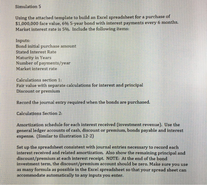
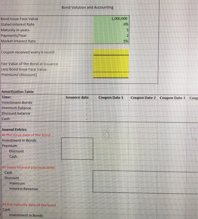
Simulation 5 Using the attached template to build an Excel spreadsheet for a purchase of $1,000,000 face value, 6% 5-year bond with interest payments every 6 months. Market interest rate is 5%. Include the following items: Inputs: Bond initial purchase amount Stated Interest Rate Maturity in Years Number of payments/year Market interest rate Calculations section 1: Fair value with separate calculations for interest and principal Discount or premium Record the journal entry required when the bonds are purchased. Calculations Section 2: Amortization schedule for each interest received (investment revenue). Use the general ledger accounts of cash, discount or premium, bonds payable and interest expense. (Similar to illustration 12-2) Set up the spreadsheet consistent with journal entries necessary to record each interest received and related amortization. Also show the remaining principal and discount/premium at each interest receipt. NOTE: At the end of the bond investment term, the discount/premium account should be zero. Make sure you use as many formula as possible in the Excel spreadsheet so that your spread sheet can accommodate automatically to any inputs you enter. Bond Valution and Accounting 1,000,000 6% Bond Issue Face Value Stated Interest Rate Maturity in years Payments/Year Market Interest Rate RN Coupon received every 6 month Fair Value of the Bond at Issuance Less Bond Issue Face Value Premium/ (Discount) Issuance date Coupon Date 1 Coupon Date 2 Coupon Date 3 Cour Amortization Table Time: Investment Bonds Preimum balance Discount balance Cash Journal Entries At the issue date of the bond Investment in Bonds Premium Discount Cash At every interest payment date: Cash Discount Premium Interest Revenue At the maturity date of the bond Cash Investment in Bonds