solve the question

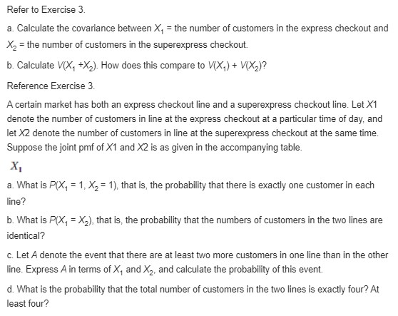
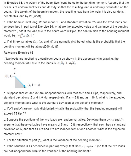
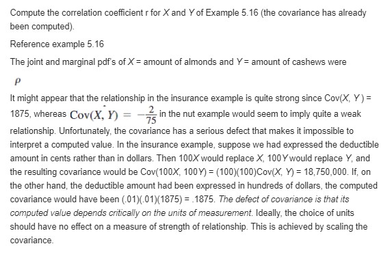
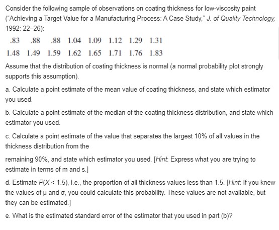
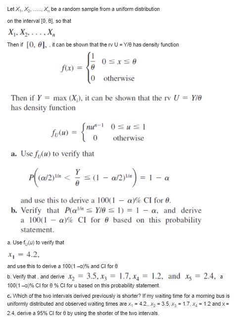
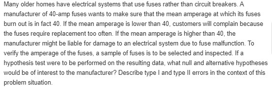
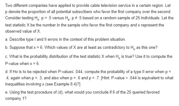
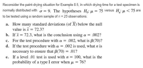
Refer to Exercise 3. a. Calculate the covariance between X, = the number of customers in the express checkout and X- = the number of customers in the superexpress checkout. b. Calculate V(X, +X,). How does this compare to V(X,) + V(X2)? Reference Exercise 3. A certain market has both an express checkout line and a superexpress checkout line. Let X1 denote the number of customers in line at the express checkout at a particular time of day, and let X2 denote the number of customers in line at the superexpress checkout at the same time. Suppose the joint pmf of X1 and X2 is as given in the accompanying table. X a. What is P(X, = 1, X, = 1), that is, the probability that there is exactly one customer in each line? b. What is P(X, = X,), that is, the probability that the numbers of customers in the two lines are identical? c. Let A denote the event that there are at least two more customers in one line than in the other line. Express A in terms of X, and X2, and calculate the probability of this event. d. What is the probability that the total number of customers in the two lines is exactly four? At least four?In Exercise 66, the weight of the beam itself contributes to the bending moment. Assume that the beam is of uniform thickness and density so that the resulting load is uniformly distributed on the beam. If the weight of the beam is random, the resulting load from the weight is also random; denote this load by W (kip-ft). a. If the beam is 12 ft long, Whas mean 1.5 and standard deviation .25, and the fixed loads are as described in part (a) of Exercise 66, what are the expected value and variance of the bending moment? [Hint: If the load due to the beam were w kip-ft, the contribution to the bending moment would be w xdx.] ] b. If all three variables (X1, X2, and W) are normally distributed, what is the probability that the bending moment will be at most200 kip-ft? Reference Exercise 66 If two loads are applied to a cantilever beam as shown in the accompanying drawing, the bending moment at 0 due to the loads is a, X, + a,X2. (0, 1)- (x, 1 - x) a. Suppose that X1 and X2 are independent rv's with means 2 and 4 kips, respectively, and standard deviations .5 and 1.0 kip, respectively. If a, = 5 ft and a2 _ 10 ft, what is the expected bending moment and what is the standard deviation of the bending moment? b. If X1 and X2 are normally distributed, what is the probability that the bending moment will exceed 75 kip-ft? c. Suppose the positions of the two loads are random variables. Denoting them by A, and A2, assume that these variables have means of 5 and 10 ft, respectively, that each has a standard deviation of .5, and that all Aj's and Xi's are independent of one another. What is the expected moment now? d. For the situation of part (c), what is the variance of the bending moment? e. If the situation is as described in part (a) except that Corr(X,, X2) = .5 (so that the two loads are not independent), what is the variance of the bending moment?Compute the correlation coefficient r for X and Y of Example 5.16 (the covariance has already been computed). Reference example 5.16 The joint and marginal pdf's of X = amount of almonds and Y = amount of cashews were D It might appear that the relationship in the insurance example is quite strong since Cov(X, Y ) = 1875, whereas Cov(X, n) = - in the nut example would seem to imply quite a weak relationship. Unfortunately, the covariance has a serious defect that makes it impossible to interpret a computed value. In the insurance example, suppose we had expressed the deductible amount in cents rather than in dollars. Then 100X would replace X, 100 Y would replace Y, and the resulting covariance would be Cov(100X, 100Y) = (100)(100)Cov(X, Y) = 18,750,000. If, on the other hand, the deductible amount had been expressed in hundreds of dollars, the computed covariance would have been (.01)(.01)(1875) = .1875. The defect of covariance is that its computed value depends critically on the units of measurement. Ideally, the choice of units should have no effect on a measure of strength of relationship. This is achieved by scaling the covariance.Consider the following sample of observations on coating thickness for low-viscosity paint ("Achieving a Target Value for a Manufacturing Process: A Case Study," J. of Quality Technology, 1992: 22-26): .83 .88 .88 1.04 1.09 1.12 1.29 1.31 1.48 1.49 1.59 1.62 1.65 1.71 1.76 1.83 Assume that the distribution of coating thickness is normal (a normal probability plot strongly supports this assumption). a. Calculate a point estimate of the mean value of coating thickness, and state which estimator you used. b. Calculate a point estimate of the median of the coating thickness distribution, and state which estimator you used. c. Calculate a point estimate of the value that separates the largest 10% of all values in the thickness distribution from the remaining 90%, and state which estimator you used. [Hint. Express what you are trying to estimate in terms of m and s.] d. Estimate P(X .044 is equivalent to what inequalities involving x (see Example 8.4)?] e. Using the test procedure of (d), what would you conclude if 6 of the 25 queried favored company 1?Reconsider the paint-drying situation for Example 8.5, in which drying time for a test specimen is normally distributed with or = 9. The hypotheses Hou = 75 versus Hou