solve this and show the formulas used
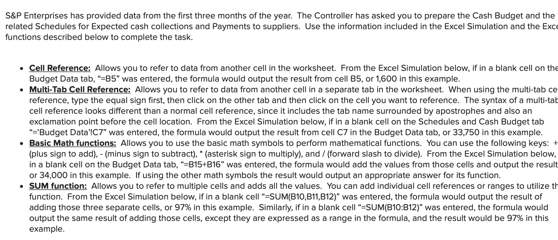
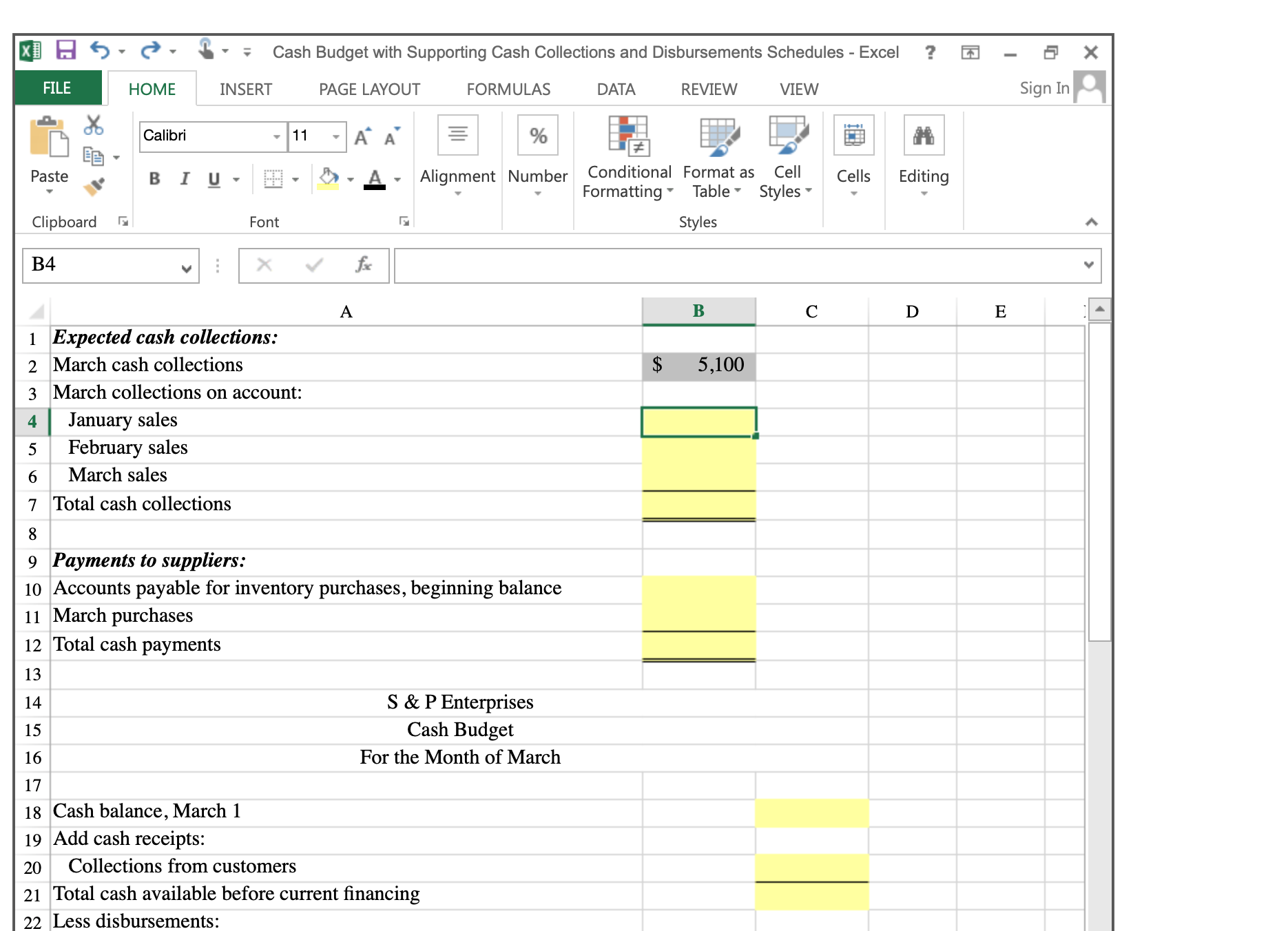
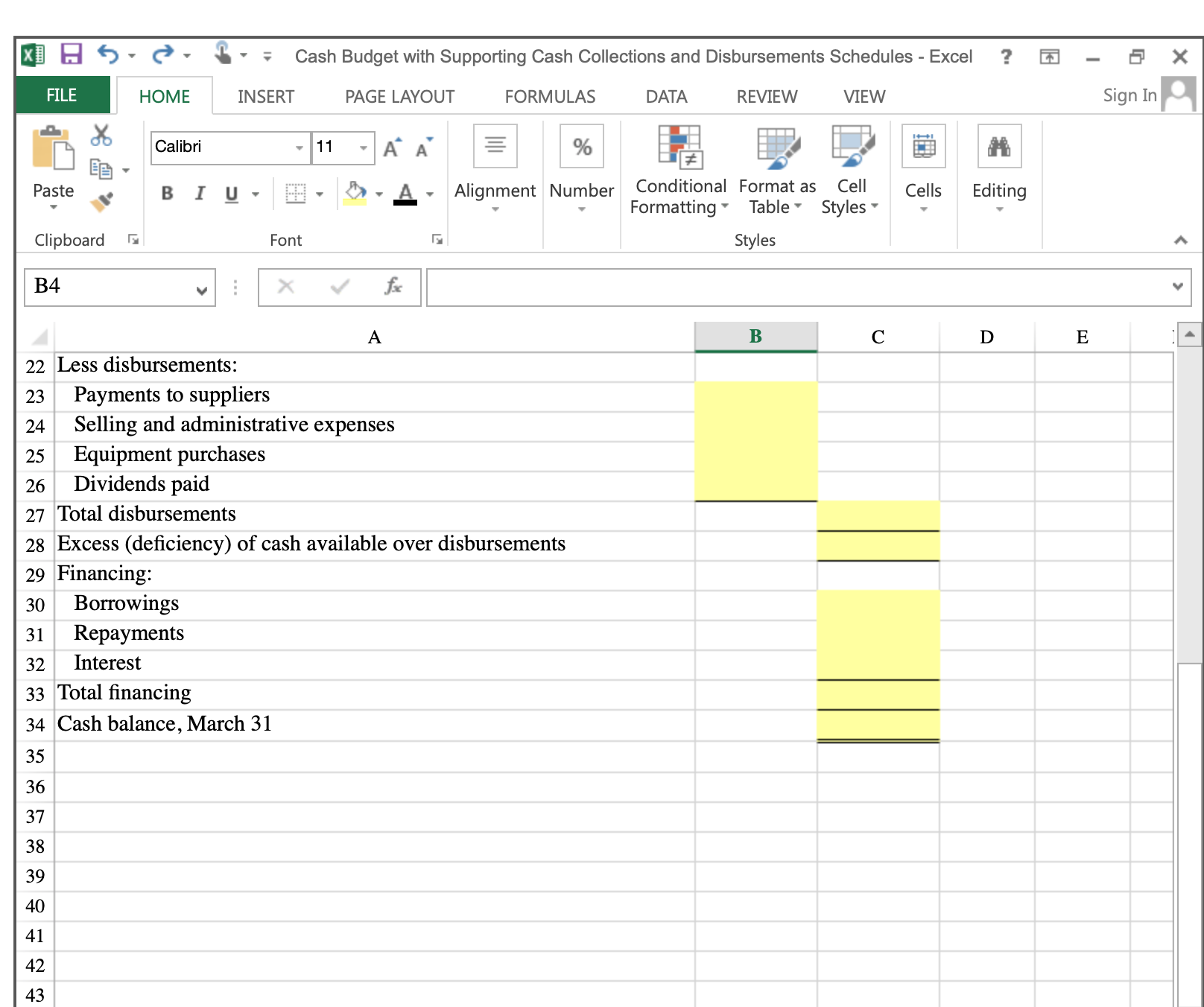
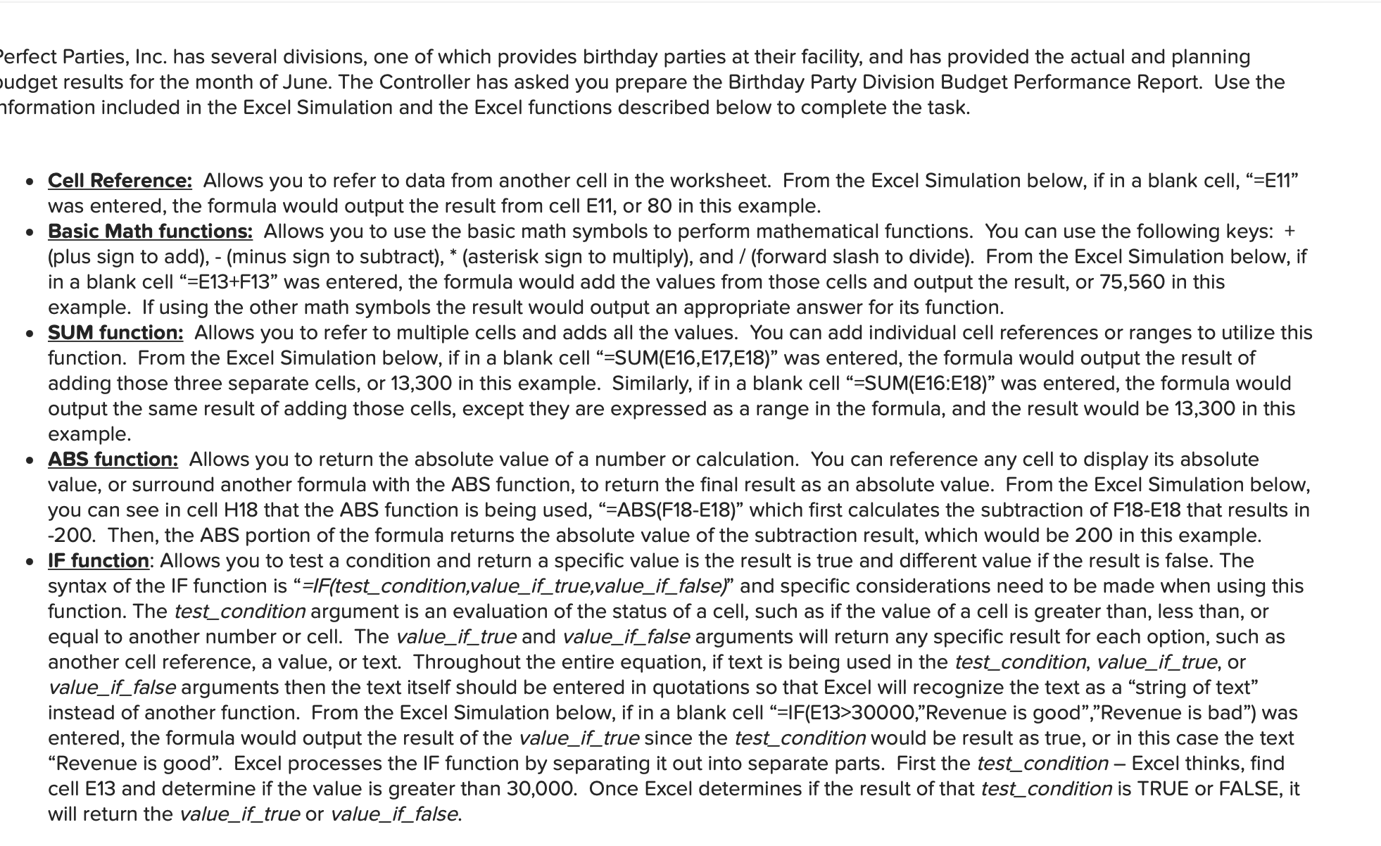
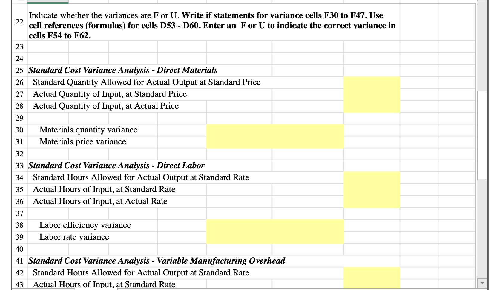
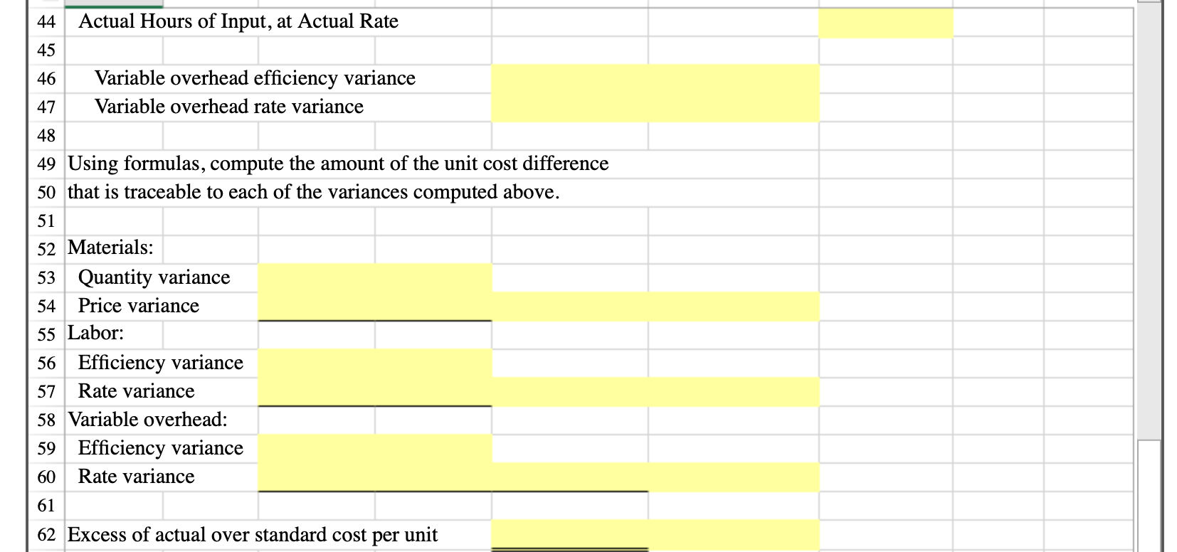
S&P Enterprises has provided data from the rst three months of the year. The Controller has asked you to prepare the Cash Budget and the related Schedules for Expected cash collections and Payments to suppliers. Use the information included in the Excel Simulation and the Exce functions described below to complete the task. - Cell Reference: Allows you to refer to data from another cell in the worksheet. From the Excel Simulation below, if in a blank cell on the Budget Data tab, \"=35" was entered, the formula would output the result from cell BS, or 1,600 in this example. - Multi-Tab Cell Reference: Allows you to refer to data from another cell in a separate tab in the worksheet. When using the multi-tab ce reference, type the equal sign first, then click on the other tab and then click on the cell you want to reference. The syntax of a multi-tal: cell reference looks different than a normal cell reference, since it includes the tab name surrounded by apostrophes and also an exclamation point before the cell location. From the Excel Simulation below, if in a blank cell on the Schedules and Cash Budget tab \"='Budget Data'!C7" was entered, the formula would output the result from cell C7 in the Budget Data tab, or 33,750 in this example. a Basic Math functions: Allows you to use the basic math symbols to perform mathematical functions. You can use the following keys: + (plus sign to add), - (minus sign to subtract), * (asterisk sign to multiply), and / (forward slash to divide). From the Excel Simulation below, in a blank cell on the Budget Data tab, \"=B15+B16\" was entered, the formula would add the values from those cells and output the result or 34,000 in this example. If using the other math symbols the result would output an appropriate answer for its function. . SUM function: Allows you to refer to multiple cells and adds all the values. You can add individual cell references or ranges to utilize ti\" function. From the Excel Simulation below, if in a blank cell \"=SUM(B10,B11,B12)\" was entered, the formula would output the result of adding those three separate cells, or 97% in this example. Similarly, if in a blank cell \"=SUM(B10:B12)\" was entered, the formula would output the same result of adding those cells, except they are expressed as a range in the formula, and the result would be 97% in this example. E '3 ' C, ' 3 ' 3 Cash Budget with Supporting Cash Collections and Disbursements Schedules- Excel ? E X FILE HOME INSERT PAGE LAVOUT FORMULAS DATA REVIEW VIEW Sign In R n- 34, .H. E at e an D Ea . .4 E Paste v B I u . . {3'9 . A . Alignment Number conditional Format as Cell Cells Editing - s v . Formatting ' Table ' Styles ' . v Clipboard G Font i?- Styles A B4 v 3 > .0" fr " Expected cash collections: March cash collections _ 1 2 3 March collections on account: n January sales I l 5 February sales 5 March sales 7 8 9 10 Total cash collections Payments to suppliers: Accounts payable for inventory purchases, beginning balance 11 March purchases 12 Total cash payments 13 14 S & P Enterprises 15 Cash Budget 16 For the Month of March 17 18 Cash balance, March 1 19 Add cash receipts: 20 Collections from customers 21 Total cash available before current nancing 22 Less disbursements: x] H 6 . . . : Cash Budget with Supporting Cash Collections and Disbursements Schedules - Excel - 5 X FILE HOME INSERT PAGE LAYOUT FORMULAS DATA REVIEW VIEW Sign In Calibri 11 AA % Paste BIU - Alignment Number Conditional Format as Cell Cells Editing Formatting * Table Styles Clipboard Font G Styles B4 X V fx A B C D E 22 Less disbursements: 23 Payments to suppliers 24 Selling and administrative expenses 25 Equipment purchases 26 Dividends paid 27 Total disbursements 28 Excess (deficiency) of cash available over disbursements 29 Financing: 30 Borrowings 31 Repayments 32 Interest 33 Total financing 34 Cash balance, March 31 35 36 37 38 39 40 41 42 43erfect Parties, Inc. has several divisions, one of which provides birthday parties at their facility, and has provided the actual and planning budget results for the month of June. The Controller has asked you prepare the Birthday Party Division Budget Performance Report. Use the formation included in the Excel Simulation and the Excel functions described below to complete the task. . Cell Reference: Allows you to refer to data from another cell in the worksheet. From the Excel Simulation below, if in a blank cell, "=E11" was entered, the formula would output the result from cell E11, or 80 in this example. . Basic Math functions: Allows you to use the basic math symbols to perform mathematical functions. You can use the following keys: + (plus sign to add), - (minus sign to subtract), *(asterisk sign to multiply), and / (forward slash to divide). From the Excel Simulation below, if in a blank cell "=E13+F13" was entered, the formula would add the values from those cells and output the result, or 75,560 in this example. If using the other math symbols the result would output an appropriate answer for its function. . SUM function: Allows you to refer to multiple cells and adds all the values. You can add individual cell references or ranges to utilize this function. From the Excel Simulation below, if in a blank cell "=SUM(E16,E17,E18)" was entered, the formula would output the result of adding those three separate cells, or 13,300 in this example. Similarly, if in a blank cell "=SUM(E16:E18)" was entered, the formula would output the same result of adding those cells, except they are expressed as a range in the formula, and the result would be 13,300 in this example. . ABS function: Allows you to return the absolute value of a number or calculation. You can reference any cell to display its absolute value, or surround another formula with the ABS function, to return the final result as an absolute value. From the Excel Simulation below, you can see in cell H18 that the ABS function is being used, "=ABS(F18-E18)" which first calculates the subtraction of F18-E18 that results in -200. Then, the ABS portion of the formula returns the absolute value of the subtraction result, which would be 200 in this example. . IF function: Allows you to test a condition and return a specific value is the result is true and different value if the result is false. The syntax of the IF function is "=/F(test_condition,value_if_true,value_if_false)" and specific considerations need to be made when using this function. The test_condition argument is an evaluation of the status of a cell, such as if the value of a cell is greater than, less than, or equal to another number or cell. The value_if_true and value_if_false arguments will return any specific result for each option, such as another cell reference, a value, or text. Throughout the entire equation, if text is being used in the test_condition, value_if_true, or value_if_false arguments then the text itself should be entered in quotations so that Excel will recognize the text as a "string of text" instead of another function. From the Excel Simulation below, if in a blank cell "=IF(E13>30000,"Revenue is good","Revenue is bad") was entered, the formula would output the result of the value_if_true since the test_condition would be result as true, or in this case the text "Revenue is good". Excel processes the IF function by separating it out into separate parts. First the test_condition - Excel thinks, find cell E13 and determine if the value is greater than 30,000. Once Excel determines if the result of that test_condition is TRUE or FALSE, it will return the value_if_true or value_if_false.Preparing a Performance Report - Excel ? 6 - X FILE HOME INSERT PAGE LAYOUT FORMULAS DATA REVIEW VIEW Sign In Calibri 11 A" A % Paste BIU - - - A . Alignment Number Conditional Format as Cell Cells Editing Formatting * Table Styles Clipboard Font Styles Al X V Perfect Parties, Inc. has several divisions. One division provides birthday parties v A B C D E F G H I J K Perfect Parties, Inc. has several divisions. One division provides birthday parties at their facility. N Each party sold provides entertainment, decorations, food, and party favors for 10 children. The bookkeeper has prepared a report comparing actual results for the month of June to budgeted results. Perfect Parties Birthday Party Division Analysis of Revenues and Costs For the Month Ended June 30 8 Planning Budget Actual Results Variances 10 11 Number of parties 80 92 12 13 Revenue $ 36,000 $ 39,560 $ 3,560 F 14 Expenses: 15 Food costs 7,200 8,648 1,448 U 16 Party supplies 3,200 3,404 204 U 17 Party worker wages 6,400 7,728 1,328 U 18 Administrative salaries 3,700 3,500 200 F 19 Equipment depreciation 1,200 1,200 None 20 Rent 5,000 5,000 None 21 Total expense 26,700 29,480 2,780 U 22 Net operating income $ 9,300 $ 10,080 $ 780 F23 Food costs, party supplies and party worker wages are variable costs. 24 Administrative salaries, equipment depreciation and rent are fixed costs. 25 26 Prepare a new report for June using the flexible budget approach. 27 Enter all variances as positive amounts. If there is a variance, write an IF statements to indicate if it is F or U (using capital letters). 28 If there is no variance, enter the word None. 29 Perfect Parties 30 Birthday Party Division Flexible Budget Performance Report 31 For the Month Ended June 30 32 Flexible 33 Planning Revenue and Actual Budget Activity Variances Budget Spending Variances Results 34 Number of parties 35 36 Revenues 37 Expenses: 38 Food costs 39 Party supplies 40 Party worker wages 41 Administrative salaries 42 Equipment depreciation 43 Rent\fPatterson, Inc. has provided details of its actual cost data for the month. The Controller has asked you to compute the basic variances and the impact of those variances on unit costs. Use the information included in the Excel Simulation and the Excel functions described below to complete the task. - Cell Reference: Allows you to refer to data from another cell in the worksheet. From the Excel Simulation below, if in a blank cell, \"=D4" was entered, the formula would output the result from cell D4, or 2.75 in this example. - Basic Math functions: Allows you to use the basic math symbols to perform mathematical functions. You can use the following keys: + (plus sign to add), - (minus sign to subtract), * (asterisk sign to multiply), and / (fonNard slash to divide). From the Excel Simulation below, if in a blank cell \"=F4+GS\" was entered, the formula would add the values from those cells and output the result, or 14.70 in this example. If using the other math symbols the result would output an appropriate answer for its function. - SUM function: Allows you to refer to multiple cells and adds all the values. You can add individual cell references or ranges to utilize this function. From the Excel Simulation below, if in a blank cell \"=SUM(D4,D5)\" was entered, the formula would output the result of adding those two separate cells, or 5.45 in this example. Similarly, if in a blank cell "=SUM(D4:D5)" was entered, the formula would output the same result of adding those cells, except they are expressed as a range in the formula, and the result would be 5.45 in this example. - ABS function: Allows you to return the absolute value of a number or calculation. You can reference any cell to display its absolute value, or surround another formula with the ABS function, to return the nal result as an absolute value. From the Excel Simulation below, if in a blank cell you entered \"=ABS(F7-68)\" Excel will rst calculate the subtraction of F7-GB that results in -0.20. Then, the ABS portion of the formula returns the absolute value of the subtraction result, which would be 0.20 in this example. - IF function: Allows you to test a condition and return a specific value is the result is true and different value if the result is false. The syntax of the IF function is \"=lF(te$t_condition,value_if_true,value_if_false)" and specic considerations need to be made when using this function. The techondition argument is an evaluation ofthe status of a cell, such as if the value ofa cell is greater than, less than, or equal to another number or cell. The value_if_true and value_if_false arguments will return any specic result for each option, such as another cell reference, a value, or text. Throughout the entire equation, if text is being used in the test_ condition, value_if_true, or value_if_false arguments then the text itself should be entered in quotations so that Excel will recognize the text as a \"string of text" instead of another function. From the Excel Simulation below, if in a blank cell "=lF(F13>20,\"Total Cost Per Unit is good\Basic Variance Analysis and the Impact of Variances on Unit Costs - Excel ? 6 - X FILE HOME INSERT PAGE LAYOUT FORMULAS DATA REVIEW VIEW Sign In Calibri 11 A A % Paste BIU - - A Alignment Number Conditional Format as Cell Cells Editing Formatting Table Styles Clipboard Font Styles A1 X V Standards for one of Patterson, Inc.'s products is shown below, along with actual A B C D E F G H I Standards for one of Patterson, Inc.'s products is shown below, along with actual cost data for the month: Direct materials: 4 Standard 2.4 yards @ $2.75 per yard $6.60 5 Actual 3 yards @ $2.70 per yard $8.10 6 Direct labor: 7 Standard 0.6 hours @ $18.00 per hour 10.80 8 Actual 0.5 hours @ $22.00 per hour 11.00 9 Variable overhead 10 Standard 0.6 hours @ $7.00 per hour 4.20 11 Actual 0.5 hours @ $7.10 per hour 3.55 12 13 Total cost per unit $21.60 $22.65 14 15 Excess of actual cost over standard cost per unit $1.05 16 17 Actual production for the month 13,500 units 18 Variable overhead is assigned to products based on direct labor hours. There 19 was no beginning or ending inventory of materials for the month. 20 Using for22 23 24 25 26 27 28 29 30 31 32 33 34 35 36 37 38 39 40 41 42 43 Indicate whether the variances are F or U. Write if statements for variance cells F30 to F47. Use cell references (formulas) for cells D53 - D60. Enter an F or U to indicate the correct variance in cells F54 to F62. Standard Cost Variance Analysis - Direct Materials Standard Quantity Allowed for Actual Output at Standard Price Actual Quantity of Input, at Standard Price Actual Quantity of Input, at Actual Price Materials quantity variance Materials price variance Standard Cost Variance Analysis - Direct Labor Standard Hours Allowed for Actual Output at Standard Rate Actual Hours of Input, at Standard Rate Actual Hours of Input, at Actual Rate Labor efciency variance Labor rate variance Standard Cost Variance Analysis - Variable Manufacturing Overhead Standard Hours Allowed for Actual Output at Standard Rate Actual Hours of Input, at Standard Rate 44 Actual Hours of Input, at Actual Rate 45 46 Variable overhead efficiency variance 47 Variable overhead rate variance 48 49 Using formulas, compute the amount of the unit cost difference 50 that is traceable to each of the variances computed above. 51 52 Materials: 53 Quantity variance 54 Price variance 55 Labor: 56 Efficiency variance 57 Rate variance 58 Variable overhead: 59 Efficiency variance 60 Rate variance 61 62 Excess of actual over standard cost per unit
