Solve using MATLAB (not by paper), please provide steps, explanations, and screenshots of the code

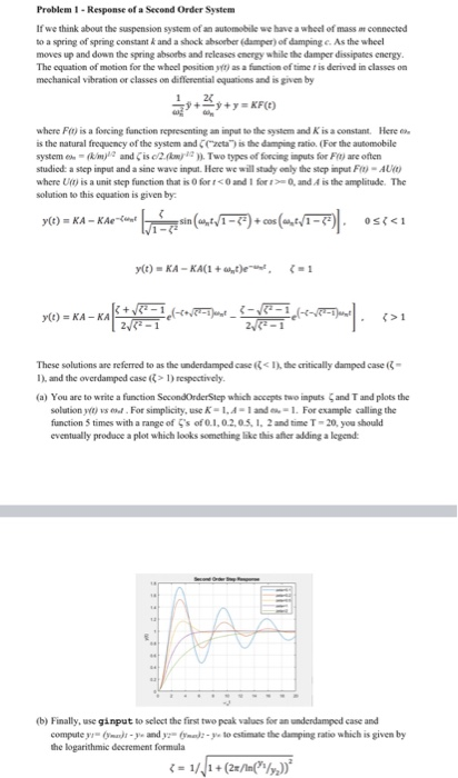
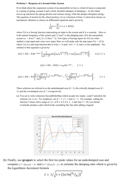
Problem 1 - Response of a Second Order System If we think about the suspension system of an automobile we have a wheel of mass connected to a spring of spring constant and a shock absorberdamper) of damping. As the wheel moves up and down the spring absorbs and releases energy while the damper dissipaties energy The equation of motion for the wheel position as a function of time is derived in classes on mechanical Vibration or classes on differential equations and is given by +23+y=KFC where is a forcing function representing an input to the system and is a constant Here is the natural frequency of the system and is the camping rate (For the automobile systems - and is c2. Two types of forcing inputs for F reeften studied a step input anda sinewave input. Here we will stay only the step input F -A where is a unit step function that is forrand fo nd is the amplitude. The solution to this equation is given by y(t) = KA - Kert h ein (29-01-3) = cos(,/1- osi(0) = xa-kali . > These solutions are referred to as the underdamped case 1)the critically damped case 1), and the overdamped case ( 1) respectively. (a) You are to write a function Second Order Step which accepts two inputs and and plots the solution yo) vs . For simplicity, use K -1.4-1 and 1. For example calling the function times with a range of 's of 0.1, 0.2.0.5. 1. 2 and time T-20, you should eventually produce a plot which looks something like this after adding a legend (b) Finally, use ginput to select the first two peal values for an underdamped case and compute y -yu and y o u to estimate the damping ratio which is given by the logarithmic decrement formula (o) Ka-kali kuwa ni pare very >> These solutions are referred to as the underdamped case 1) respectively, (a) You are to write a function SecondOrderStep which accepts two inputs and T and plots the solution y o u. For simplicity, use K-1,4-1 and 1. For example calling the function 5 times with a range of 's of 0.1, 0.2, 0.5, 1, 2 and time T-20, you should eventually produce a plot which looks something like this after adding a legend Second Onderstepona (b) Finally, use ginput to select the first two peak values for an underdamped case and compute yr ( yle and y )2-ye to estimate the damping ratio which is given by the logarithmic decrement formula 3 = 11/1+(27/In{":/y2))