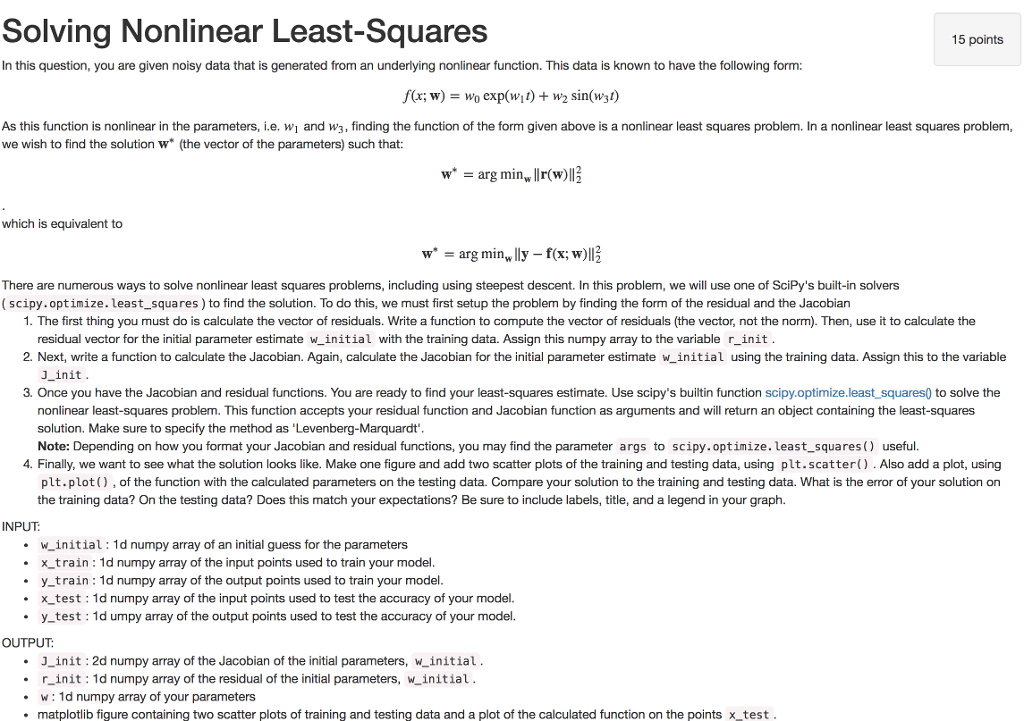
Solving Nonlinear Least-Squares 15 points In this question, you are given noisy data that is generated from an underlying nonlinear function. This data is known to have the following form: f(x; w)wo exp(wit) + w2 sin(wjt) As this function is nonlinear in the parameters, i.e. wi and w3, finding the function of the form given above is a nonlinear least squares problem. In a nonlinear least squares problem, we wish to find the solution w" (the vector of the parameters) such that: which is equivalent to w" = arg min," lly-f(x; w)11 There are numerous ways to solve nonlinear least squares problems, including using steepest descent. In this problem, we will use one of SciPy's built-in solvers (scipy.optimize. least_squares) to find the solution. To do this, we must first setup the problem by finding the form of the residual and the Jacobian 1. The first thing you must do is calculate the vector of residuals. Write a function to compute the vector of residuals (the vector, not the norm). Then, use it to calculate the 2. Next, write a function to calculate the Jacobian. Again, calculate the Jacobian for the initial parameter estimate w_initial using the training data. Assign this to the variable 3. Once you have the Jacobian and residual functions. You are ready to find your least-squares estimate. Use scipy's builtin function scipy.optimize.least squares0 to solve the residual vector for the initial parameter estimate w_initial with the training data. Assign this numpy array to the variable r_init. J_init nonlinear least-squares problem. This function accepts your residual function and Jacobian function as arguments and will return an object containing the least-squares solution. Make sure to specify the method as 'Levenberg-Marquardt' Note: Depending on how you format your Jacobian and residual functions, you may find the parameter args to scipy.optimize.least_squares() useful. 4. Finally, we want to see what the solution looks like. Make one figure and add two scatter plots of the training and testing data, using plt.scatter(). Also add a plot, using plt.plot), of the function with the calculated parameters on the testing data. Compare your solution to the training and testing data. What is the error of your solution on the training data? On the testing data? Does this match your expectations? Be sure to include labels, title, and a legend in your graph. INPUT .winitial: 1d numpy array of an initial guess for the parameters x train 1d numpy array of the input points used to train your model y_train: 1d numpy array of the output points used to train your model y_test 1d umpy array of the output points used to test the accuracy of your model. J_init : 2d numpy array of the Jacobian of the initial parameters, w initial. .x test 1d numpy array of the input points used to test the accuracy of your model OUTPUT r_init : 1d numpy array of the residual of the initial parameters, w-initial .W: 1d numpy array of your parameters matplotlib fiqure containing two scatter plots of training and testing data and a plot of the calculated function on the points x test. Solving Nonlinear Least-Squares 15 points In this question, you are given noisy data that is generated from an underlying nonlinear function. This data is known to have the following form: f(x; w)wo exp(wit) + w2 sin(wjt) As this function is nonlinear in the parameters, i.e. wi and w3, finding the function of the form given above is a nonlinear least squares problem. In a nonlinear least squares problem, we wish to find the solution w" (the vector of the parameters) such that: which is equivalent to w" = arg min," lly-f(x; w)11 There are numerous ways to solve nonlinear least squares problems, including using steepest descent. In this problem, we will use one of SciPy's built-in solvers (scipy.optimize. least_squares) to find the solution. To do this, we must first setup the problem by finding the form of the residual and the Jacobian 1. The first thing you must do is calculate the vector of residuals. Write a function to compute the vector of residuals (the vector, not the norm). Then, use it to calculate the 2. Next, write a function to calculate the Jacobian. Again, calculate the Jacobian for the initial parameter estimate w_initial using the training data. Assign this to the variable 3. Once you have the Jacobian and residual functions. You are ready to find your least-squares estimate. Use scipy's builtin function scipy.optimize.least squares0 to solve the residual vector for the initial parameter estimate w_initial with the training data. Assign this numpy array to the variable r_init. J_init nonlinear least-squares problem. This function accepts your residual function and Jacobian function as arguments and will return an object containing the least-squares solution. Make sure to specify the method as 'Levenberg-Marquardt' Note: Depending on how you format your Jacobian and residual functions, you may find the parameter args to scipy.optimize.least_squares() useful. 4. Finally, we want to see what the solution looks like. Make one figure and add two scatter plots of the training and testing data, using plt.scatter(). Also add a plot, using plt.plot), of the function with the calculated parameters on the testing data. Compare your solution to the training and testing data. What is the error of your solution on the training data? On the testing data? Does this match your expectations? Be sure to include labels, title, and a legend in your graph. INPUT .winitial: 1d numpy array of an initial guess for the parameters x train 1d numpy array of the input points used to train your model y_train: 1d numpy array of the output points used to train your model y_test 1d umpy array of the output points used to test the accuracy of your model. J_init : 2d numpy array of the Jacobian of the initial parameters, w initial. .x test 1d numpy array of the input points used to test the accuracy of your model OUTPUT r_init : 1d numpy array of the residual of the initial parameters, w-initial .W: 1d numpy array of your parameters matplotlib fiqure containing two scatter plots of training and testing data and a plot of the calculated function on the points x test