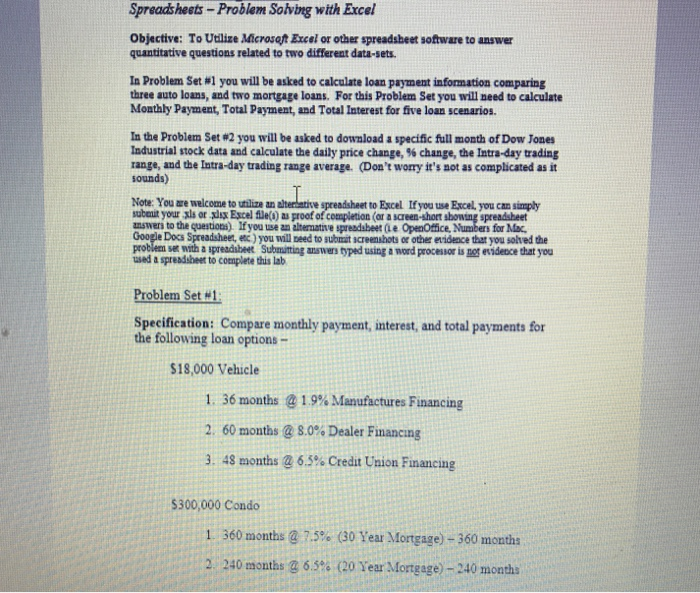
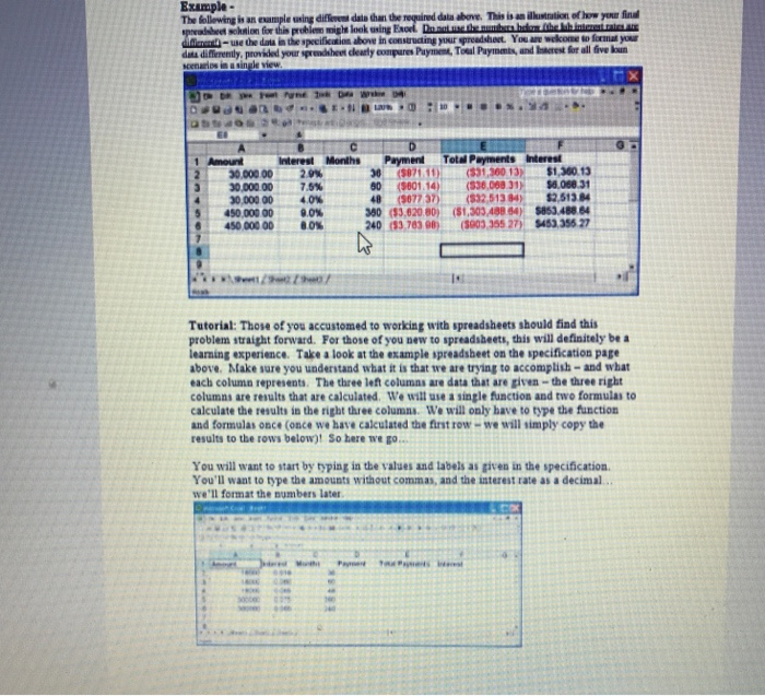
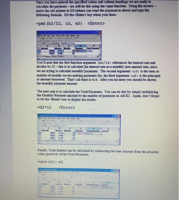
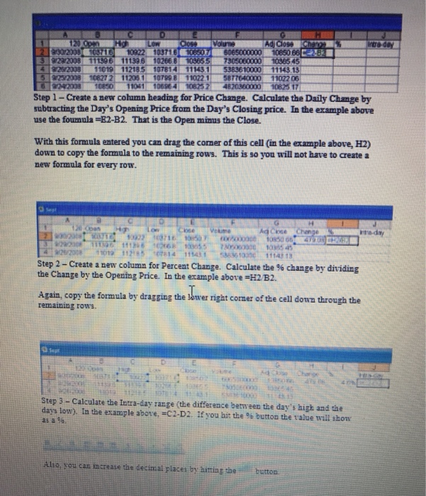
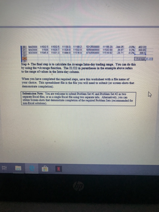
Spreadsheets- Problem Soiving with Excel Objective: To Utilize Microsoft Excel or other spreadsbeet software to answer quantitative questions related to two different data-sets. In Problem Set #1 you will be asked to calculate loan payment information comparing three auto loans, and two mortgage loans. For this Problem Set you will need to calculate Monthly Payment, Total Payment, and Total Interest for five loan scenarios In the Problem Set #2 you will be asked to download a specific full month of Dow Jones Industrial stock data and calculate the daily price change, % change, the Intra-day trading range, and the Intra-day trading range average. (Don't worry it's not as complicated as it sounds) Note: You are welcome to utilize an subenit your als or ylx Excel file) as proof of completion (ar a screen-short mswers to the guestions) If you use an alternative spreadsheet (Le OpenOffice spreadsheet to Excel If you use Excel, you can simply spreadsheet s for Mac Docs Spreadsheet, ec) you will seed to submit screenshots or othe eridence that you solved the ser with a spreadsbeet Submuitting answers typed using a word processor is nos evidence that you used a spreadsheet to complete this lab Problem Set #1 Specification: Compare monthly payment, interest, and total payments for the following loan options $18,000 Vehicle 1. 36 months @ 1 9% Manufactures Financing 2. 60 months @ 8.0% Dealer Financing 3. 4S months @ 6.5% Credit Union Financing 5300,000 Condo 1. 360 months @ 7.5% (30 Year Mortgage)-360 months 2 2 40 months @ 6.5% (20 Year Mortgage)-240 months Example The follewing is an example using diflevess daia than the required daia above. This isan ilkustration ofhow yo final -ue dhe data in the specificotios abone in consuucting yiur spreadshest. You are welcome to format your 1 Amount Interest Months Payment Total Payments Iinterest (5871.11)($31,360 13$1,300.1 30,00000 30,00000 30000 00 450 000 00 450 00000 29% 75% 40% 90% 80% 0 (5601.14)(336,068 31$6.068 31 0 9077 37)832 513 9$2,513 0 (33,620 80) (1,303,488 64) 5853.488 64 240 (3,76390)5003,355 27) 453356 27 Tutorial: Those of you accustomed to working with spreadsheets should find this problem straight forward. For those of you new to spreadsheets, this will definitely be a learning experience. Take a look at the example spreadsbeet on the specification page above. Make sure you understand what it is that we are trying to accomplish and what each column represents. The three left columas are data that are given-the three right columas are results that are calculated. We will use a single function and two formulas to calculate the results in the right three columns. We will only have to type the function and formulas once (once we have calculated the first row-we will simply copy the results to the rows below)! So here e go You will want to start by typing in the values and labels as given in the specification. You'll want to type the amounts without commas, and the interest rate as a decimal we'll format the numbers later calculate the payment-we will do this using the -put function. Using the arrows- move the cell pointer to D2 (wbere you want the payment to show) and type the following formula. 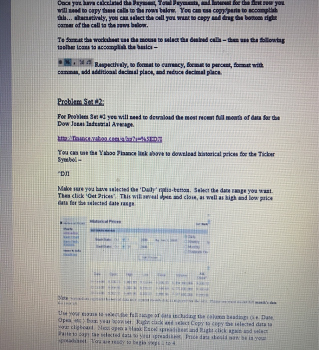Hit the Enter key when your done -pmt (b2/12, c2, a2) You'll note that the first function argument (b2/12) references the interest rate and divides by 12-this is to calculate he interest rate as a monthly (not annual) rate, since we are trying to calculate number of months we are making payments for, the third argument (a2) is the principal or amount borrowed. That's all there is to it After you hit enter you should be show the monthly payment amount. The second argument (c2) is the term or The next step is to calculate the Total Payments. You can do this by simply multiplying the Monthly Payment amount by the sumber of payments in cell E2. Again, don't forget to hit the Firally, Total Interest can be calculated by subtracting the loan Amount from the absolute value (positive) of the Total Payments abs (e2)-32 Oacs you have calcltad the Paymant, Total Prymt, nd Intarest for tan ast row yon will seed to copy thase calls to tha rows balow. You can use copy/paste to accomplsh this... ataraatively, you cn salect the call you want to copy and drng the botton right cornar of the call to tha rows balow To format the wozlkhnt uss the mouse to velact the destred calls-tha use tha followiag toolbar icons to accomplish tha basics- Respectivaly, to format to currency, format to parceat, format with commas, add additional dacimal place, and reduce decimal place. Problem Set 2: For Problem Set #2 you will need to download the most recent full month of data for the Dow Jones Industrial Average. You can use the Yahoo Finance link above to dowaload historical prices for the Ticker Symbol- Make sure you have selected the 'Daily' rpdio-button. Select the date range you want. Then click Get Prices'. This will reveal open and close, as well as high and low price data for the selected date range. it Note Use your mouse to select dhe full zange of data including te columa beadings (ie. Date, Open, e%) from your browser Ritt cick and select Copy to copy the selected data to your cligboard Next open a blanx Excel spreadsheet and Right click again and select te to opy the kelected data to your spreadsheet. Price data shoald aow be in your epreadsheet Hou are ready to begia steps 1 to 4 9252038 11019112185 OT61411143153836 10000 1114313 2 112051 1079110221 587640000 302206 Step 1- Create a new cohumn heading for Price Change. Calculate the Daily Change by subtracting the Day's Opening Price from the Day's Closing price. In the example above use the foumula B2-B2. That is the Open minus the Close. With this formula entered you can drag the comer of this cell (in the example above, H2) down to copy the formula to the remaining rows. This is so you will not have to create a new formula for every row Step 2-Create a new column for Percent Change. Calculate the % change by dividing the Change by the Opening Price. In the example above -H2 B2. Again, copy the formula by drag ging the lkawer right cormer of the cell dowa through the remaining rows Step 3- Calculate the Intra-day range (the difference betwyeen the day's high and tae days low). I the example above,-c2-D2. If you hit the % button the rate hor o you can increase ths decimal places by himing the buttoa. Step 4- The final step is to calculate the Average Intra-day trading range. You can do this by using the -Average function. The 12:322 in parentheses in the example above refers to the range of values in the Intra-day column. When you have completed the required steps, save this worksbeet with a file name of your choice. This spreadsheet file is the file you will need to submit (or screen-shots that demonstrate completion) Submision Note: You are welcome to subeit Problem Ser 1 and Probiem Ser2 as wo separate Excel files, or as a single Esxcel file uning two veparate tabs. Altemarively, you can utilize Screen-shots that demonstrate complerion of the required Probiem Sets (recommended for non-Excel solutions) t