

Answered step by step
Verified Expert Solution
Question
1 Approved Answer
Start Excel. Open exploring_ecap_grader_c2_Transactions.xlsx and save the workbook as exploring_ecap_grader_c2_Transactions_LastFirst . 0 2 On the JuneTotals worksheet, sort the data in the range A3:E16 in
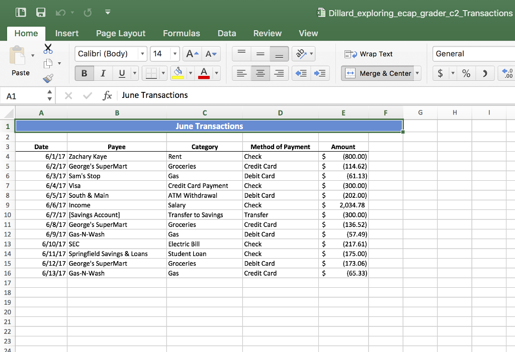 Start Excel. Open exploring_ecap_grader_c2_Transactions.xlsx and save the workbook asexploring_ecap_grader_c2_Transactions_LastFirst. Start Excel. Open exploring_ecap_grader_c2_Transactions.xlsx and save the workbook asexploring_ecap_grader_c2_Transactions_LastFirst. | 0 | |
| 2 | On the JuneTotals worksheet, sort the data in the range A3:E16 in ascending order by Category. At each change in Category, use the Sum function to add subtotals to the data in the Amount column. Accept all other defaults. Collapse the outline to show the grand total and Category subtotals only. | 4 |
| 3 | Create a PivotTable in cell F1 on the AnnualExp worksheet using the data in the range A1:D17. Add the Expense field to the PivotTable as a row label; add the Amount field as the value; add the Year field as the column label. Change the format of the values in the PivotTable to accounting with no decimal places and set columns F:J to AutoFit Column Width. | 4 |
| 4 | Add the Category field to the Report Filter area of the PivotTable. Filter the data so that only expenses in the Variable category are displayed. Display the values as percentages of the grand total. | 4 |
| 5 | Insert a Year slicer in the worksheet and use the slicer to filter the data so that only data from 2015 is displayed. Change the height of the slicer to 2" and then reposition it so that the top left corner aligns with the top left corner of cell I2. | 4 |
| 6 | Create a PivotChart based on the data in the PivotTable using the default Pie chart type. Change the chart title text to Variable Expensesand remove the legend. Add data labels to the outside end position displaying only the category names and leader lines. Reposition the chart so that the top left corner aligns with the top left corner of cell F13. Note, Mac users, select the range F5:G7, and on the Insert tab, click Pie, and then click Pie. Follow the remaining instructions. | 4 |
| 7 | On the HomeLoan worksheet, in cell A10, enter a reference to the monthly payment from column B. Create a one-variable data table for the range A9:H10 using the interest rate from column B as the Row input cell. | 4 |
| 8 | On the HomeLoan worksheet, in cell A12, enter a reference to the monthly payment from column B. Create a two-variable data table in the range A12:H16, using the interest rate from column B as the Row input cell and the term in months from column B as the Column input cell. | 4 |
| 9 | On the HomeLoan worksheet, perform a goal seek analysis to determine what the down payment in column B needs to be if you want the monthly payment in column B to be 2000. Accept the solution. | 4 |
| 10 | On the HomeLoan worksheet, create a scenario named Maximum using cells B2, B3, B5, and B6 as the changing cells. Enter these values for the scenario:280000, 24000, .075, and 360, respectively. Show the results and close the Scenario Manager. Undo the last change. | 4 |
| 11 | On the June2017 worksheet, in cell I7, sum the values in E7:E24 if the purchase in column C is groceries; in cell I8, average the values in E7:E24 if the purchase in column C is groceries; in cell I9, calculate the number of times groceries were purchased during the month. | 9 |
| 12 | On the June2017 worksheet, in cell I11, calculate the total amount spent on groceries using a credit card; in cell I12, calculate the average spent on groceries using a credit card; in cell I13, calculate the number of times groceries were purchased using a credit card during the month. | 9 |
| 13 | On the June2017 worksheet, in cell F7, nest an AND function within an IF function to determine if the transaction was paid using a credit card and the amount of the transaction is less than-100. If both conditions are met in the AND function, the function should return the text Flag. For all others, the function should return the text OK. Copy the function down through cell F24. | 6 |
| 14 | On the June2017 worksheet, in cell E4, use the INDEX function to identify the transaction amount that aligns with the position in cell C4. Type 5 for the column_num and use the range A7:E24 as the array argument. | 6 |
| 15 | On the June2017 worksheet, filter the data in the range A6:E24 using the criteria in the range A27:E28. Set the filter to copy the data to the range A31:E31. In cell I17, use the DAVERAGE function to determine the average amount spent for transactions meeting the criteria in the range A27:E28. | 4 |
| 16 | Group the June2017 and JuneTotals worksheets together. Fill the contents and formatting from cell A1 on the JuneTotals worksheet across the grouped worksheets. Ungroup the worksheets. In cell I19 on the June2017 worksheet, insert a reference to cell E26 on the JuneTotals worksheet. | 3 |
| 17 | On the June2017 worksheet, create a validation rule for the range D7:D24 to only allow values in the list from the range I21:I24. Create an error alert for the rule that will display after invalid data is entered. Using the Stop style, enter Invalid Entry as the title and Please select a valid method. (including the period) as the error message. | 5 |
| 18 | On the CarLoan worksheet, in cell G10, use the CUMPRINC function to calculate the cumulative principle paid on the car loan. Use the data in the range E4:E6 when entering the first three arguments in the function. Reference cell A10 as the start and end period arguments. Enter 0 as the type argument. Modify the function to convert the results to a positive value. Make the row references absolute in all arguments except for the end period. Copy the formula down through cell G19. | 6 |
| 19 | From Excel, open the downloaded tab-delimited text file eV2_stocks.txt using a data format of general. You do not need to create a connection to the original data file. Copy the range A1:F5 and then close the text file. Paste the copied range onto the Stocks worksheet in cell A3. | 4 |
| 20 | On the Stocks worksheet, separate the text in the first column into two columns using the asterisk (*) as the delimiter. Insert a function in cell A3 that will display the text in cell A9 with initial capitalization only. | 4 |
| 21 | On the Stocks worksheet, import the downloaded XML file eV2_highclose.xml into cell A11. Open the XML file in Notepad, and then find and replace all instances of the text General Electric with General Electric Co (no period). Save the XML document and close Notepad. Refresh the XML data on the Stocks worksheet. Note, Mac users, import the comma-delimitedeV2_highclose.csvfile into cell A11. Open the CSV file in Excel, and then find and replace all instances of the text General Electric with General Electric Co (no period). Save and close the CSV document. Refresh the data on the Stocks worksheet. | 4 |
| 22 | Apply the Retrospect theme to the workbook. Apply the cell style Accent1 to cells A3 and D3 on the CarLoan worksheet. | 2 |
| 23 | Set the Author property of the workbook to Exploring Excel Student and then set the Title property toPersonal Finances. | 2 |
| 24 | Save the workbook. Ensure that the following worksheets are present (in this order): JuneTotals, June2017, AnnualExp, HomeLoan, CarLoan, Stocks. Close the workbook, and then submit the file as directed. |
Step by Step Solution
There are 3 Steps involved in it
Step: 1

Get Instant Access to Expert-Tailored Solutions
See step-by-step solutions with expert insights and AI powered tools for academic success
Step: 2

Step: 3
Ace Your Homework with AI
Get the answers you need in no time with our AI-driven, step-by-step assistance
Get Started
Data Science For Dummies
Authors: Lillian Pierson ,Jake Porway
2nd Edition
1119327636, 978-1119327639