| Step | Instructions |
| 1 | Start Excel. Download and open the file named Exp19_Excel_Ch07_CapAssessment_Shipping.xlsx. Grader has automatically added your last name to the beginning of the filename. |
| 2 | The Week worksheet contains data for the week of April 5. In cell D7, insert the appropriate date function to calculate the number of days between the Date Arrived and Date Ordered. Copy the function to the range D8:D35. |
| 3 | Next, you want to display the city names that correspond with the city airport codes. In cell F7, insert the SWITCH function to evaluate the airport code in cell E7. Include mixed cell references to the city names in the range F2:F4. Use the airport codes as text for the Value arguments. Copy the function to the range F8:F35. |
| 4 | Now you want to display the standard shipping costs by city. In cell H7, insert the IFS function to identify the shipping cost based on the airport code and the applicable shipping rates in the range G2:G4. Use relative and mixed references correctly. Copy the function to the range H8:H35. |
| 5 | Finally, you want to calculate a partial shipping refund if two conditions are met. In cell I7, insert an IF function with a nested AND function to determine shipping refunds. The AND function should ensure both conditions are met: Total Days is grater than Total Days Delivery Goal (cell C3) and Order Total is equal to or greater than Order Total Threshold (cell C2). If both conditions are met, the refund is 50% (cell C4) of the Shipping Cost. Otherwise, the refund is $0. Use mixed references as needed. Copy the function to the range I8:I35. |
| 6 | The Stats worksheet contains similar data. Now you want to enter summary statistics. In cell B2, insert the COUNTIF function to count the number of shipments for Austin (cell B1). Use appropriate mixed references to the range argument to keep the column letters the same. Copy the function to the range C2:D2. |
| 7 | In cell B3, insert the SUMIF function to calculate the total orders for Austin (cell B1). Use appropriate mixed references to the range argument to keep the column letters the same. Copy the function to the range C3:D3. |
| 8 | In cell B4, insert the AVERAGEIF function to calculate the average number of days for shipments from Austin (cell B1). Use appropriate mixed references to the range argument to keep the column letters the same. Copy the function to the range C4:D4. |
| 9 | Now you want to focus on shipments from Houston where the order was greater than $1,000. In cell C7, insert the COUNTIFS function to count the number of orders where the Airport Code is IAH (Cell D1) and the Order Total is greater than $1,000. |
| 10 | In cell C8, insert the SUMIFS function to calculate the total orders where the Airport Code is IAH (Cell D1) and the Order Total is greater than $1,000. |
| 11 | In cell C9, insert the MAXIFS function to return the highest order total where the Airport Code is IAH (Cell D1) and the Order Total is greater than $1,000. |
| 12 | On the Map worksheet, insert a map for the states and revenues. Cut and paste the map in cell C1. |
| 13 | Format the data series to show only regions with data and show all map labels. |
| 14 | Change the map title to April 5-9 Gross Revenue. |
| 15 | Use the Loan worksheet to complete the loan amortization table. In cell F2, insert the IPMT function to calculate the interest for the first payment. Copy the function to the range F3:F25. (The results will update after you complete the other functions and formulas.) |
| 16 | In cell G2, insert the PPMT function to calculate the principal paid for the first payment. Copy the function to the range G3:G25. |
| 17 | In cell H2, insert a formula to calculate the ending principal balance. Copy the formula to the range H3:H25. |
| 18 | Now you want to determine how much interest was paid during the first two years. In cell B10, insert the CUMIPMT function to calculate the cumulative interest after the first two years. Make sure the result is positive. |
| 19 | In cell B11, insert the CUMPRINC function to calculate the cumulative principal paid at the end of the first two years. Make sure the result is positive. |
| 20 | You want to perform a what-if analysis to determine the rate if the monthly payment is $1,150 instead of $1,207.87. In cell B15, insert the RATE function to calculate the necessary monthly rate given the NPER, proposed monthly payment, and loan. Make sure the result is positive. |
| 21 | Finally, you want to convert the monthly rate to an APR. In cell B16, insert a formula to calculate the APR for the monthly rate in cell B15. |
| 22 | Insert a footer on all sheets with your name on the left side, the sheet name code in the center, and the file name code on the right side. |
| 23 | Save and close Exp19_Excel_Ch07_CapAssessment_Shipping.xlsx. Exit Excel. Submit the file as directed. 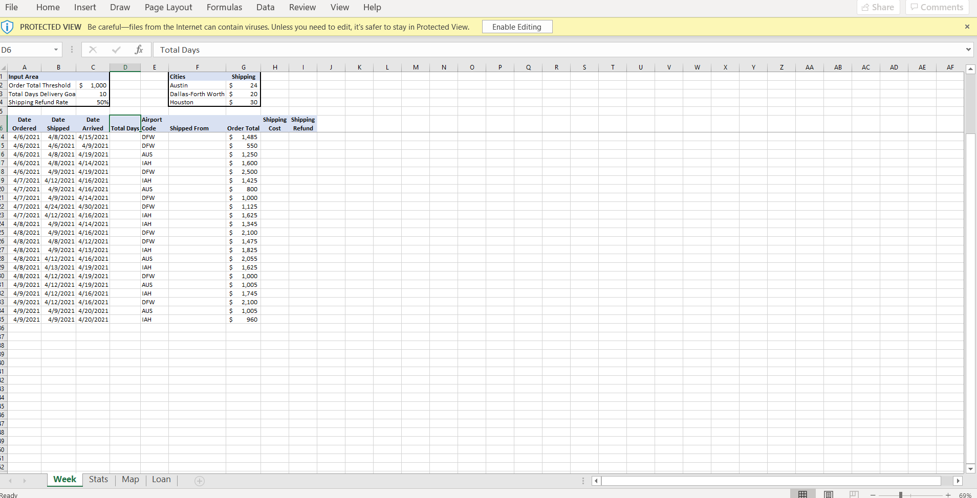 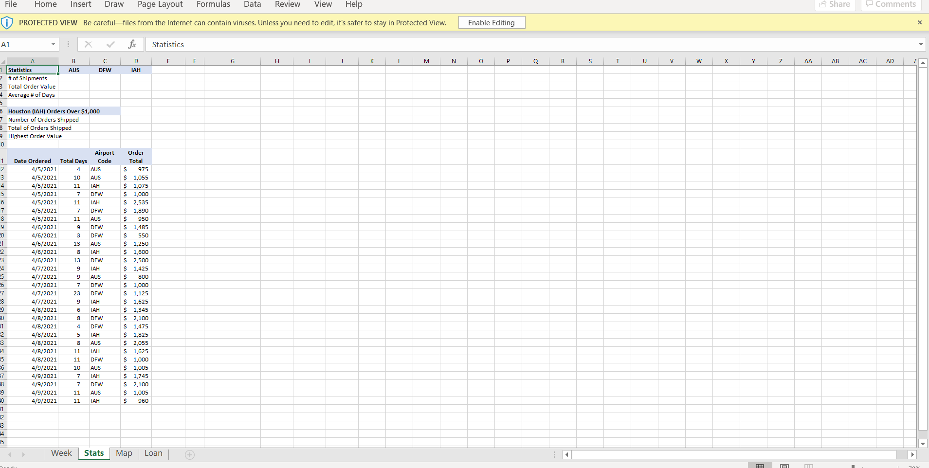 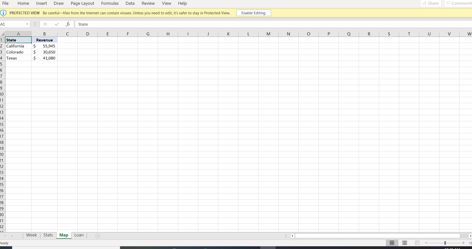 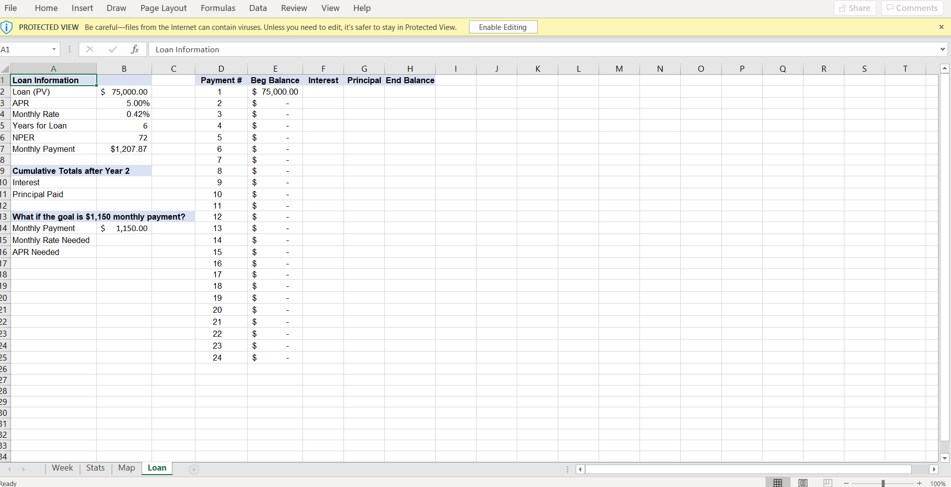
|
File Home Insert Draw Page Layout Formulas Data Review View Help Share Comments i PROTECTED VIEW Be carefulfiles from the Internet can contain viruses. Unless you need to edit, it's safer to stay in Protected View. Enable Editing X DO X fic Total Days C D E j K L M N 0 P Q R S U V w X Y Z AA AB AC AD AE AF A B 1 Input Area Order Total Threshold Total Days Delivery Goa 4 Shipping Refund Rate $ 1,000 10 50% F G Cities Shipping Austin $ 24 Dallas-Forth Worth $ 20 Houston $ 30 Shipping Shipping Cost Refund Shipped From Date Date Date Airport Ordered Shipped Arrived Total Days Code 4 4/6/2021 4/8/2021 4/15/2021 DFW 5 4/6/2021 4/6/2021 4/9/2021 DFW 6 4/6/2021 4/8/2021 4/19/2021 AUS 7 4/6/2021 4/8/2021 4/14/2021 IAH 8 4/6/2021 4/9/2021 4/19/2021 DFW 9 4/7/2021 4/12/2021 4/16/2021 IAH 0 4/7/2021 4/9/2021 4/16/2021 AUS 4/7/2021 4/9/2021 4/14/2021 DFW 2 4/7/2021 4/24/2021 4/30/2021 DFW 4/7/2021 4/12/2021 4/16/2021 24 4/8/2021 4/9/2021 4/14/2021 IAH 5 4/8/2021 4/9/2021 4/16/2021 DFW 26 4/8/2021 4/8/2021 4/12/2021 DFW 27 4/8/2021 4/9/2021 4/13/2021 IAH 28 4/8/2021 4/12/2021 4/16/2021 AUS 9 4/8/2021 4/13/2021 4/19/2021 IAH 0 4/8/2021 4/12/2021 4/19/2021 DFW 1 4/9/2021 4/12/2021 4/19/2021 AUS 2 4/9/2021 4/12/2021 4/16/2021 4/9/2021 4/12/2021 4/16/2021 DFW 4 4/9/2021 4/9/2021 4/20/2021 AUS 5 4/9/2021 4/9/2021 4/20/2021 IAH 6 7 8 9 10 1 12 13 14 15 16 Order Total $ 1,485 $ 550 S 1,250 S 1,600 $ 2,500 S 1,425 S 800 1,000 $ 1,125 $ 1,625 $ 1.345 $ 2,100 $ 1,475 S 1,825 $ 2,055 $ 1,625 $ 1,000 $ 1,005 $ 1,745 $ 2,100 $ 1,005 $ 960 18 0 1 2 Week Stats Map Loan + Ready W 69% File Home Insert Draw Page Layout Formulas Data Review View Help Share Comments PROTECTED VIEW Be carefulfiles from the Internet can contain viruses. Unless you need to edit, it's safer to stay in Protected View. Enable Editing X A1 X fr Statistics E F H J L M N 0 P O R S T V w X Y Z AA AB AC AD B AUS DFW D IAH Statistics 2 # of Shipments Total Order Value 4 Average # of Days Houston (IAH) Orders Over $1,000 Number of Orders Shipped Total of Orders Shipped 9 Highest Order Value 0 Airport Order 1 Date Ordered Total Days Code Total 2 4/5/2021 4 AUS $ 975 3 4/5/2021 10 AUS $ 1,055 4 4/5/2021 11 IAH $ 1,075 5 4/5/2021 7 DFW $1,000 6 4/5/2021 11 IAH $ 2,535 7 4/5/2021 DFW $ 1,890 8 4/5/2021 11 AUS 950 9 4/6/2021 9 DFW $ 1,485 0 4/6/2021 DFW $ 550 1 4/6/2021 13 AUS $ 1,250 2 4/6/2021 IAH $ 1,600 3 4/6/2021 13 DFW $ 2,500 24 4/7/2021 IAH $ 1,425 5 4/7/2021 9 AUS S 800 26 4/7/2021 7 DFW $ 1,000 4/7/2021 23 DFW $ 1,125 8 4/7/2021 $ 1,625 E9 4/8/2021 6 IAH $ 1,345 EO 4/8/2021 8 DFW $ 2,100 1 4/8/2021 DFW $ 1,475 2 4/8/2021 IAH 1,825 33 4/8/2021 AUS $ 2,055 4 4/8/2021 11 IAH $ 1,625 5 4/8/2021 11 DFW $ 1,000 6 4/9/2021 10 AUS $ 1,005 7 4/9/2021 IAH $ 1,745 8 4/9/2021 7 DFW $ 2,100 99 4/9/2021 11 AUS $ 1,005 10 4/9/2021 11 IAH $ 960 11 12 33 14 15 Week Stats Map Loan FRA File Home Insert Draw Page Layout Formulas Data Review View Help Share Comments i PROTECTED VIEW Be carefulfiles from the Internet can contain viruses. Unless you need to edit, it's safer to stay in Protected View. Enable Editing A1 fic State A B D E F G H 1 J K L M N o 0 R S T U V W Revenue $ 55,945 $ 30,650 $ 41,080 1 State 2 California 3 Colorado 4 Texas 5 6 7 8 9 10 11 12 13 14 15 16 17 18 19 20 21 22 23 24 25 26 27 28 29 BO 31 32 Week Stats Map Loan Ready 10 File Home Insert Draw Page Layout Formulas Data Review View Help Share Comments PROTECTED VIEW Be carefulfiles from the Internet can contain viruses. Unless you need to edit, it's safer to stay in Protected View. Enable Editing X A1 Loan Information J K L M N. o Q R S T D E F . Payment # Beg Balance Interest Principal End Balance $ 75,000.00 2 $ 3 $ 4 $ $ $ 5 6 7 8 $ $ $ 9 10 $ $ 11 12 13 $ $ 14 $ 15 $ 16 $ B 1 Loan Information 2 Loan (PV) $ 75,000.00 3 APR 5.00% 4 Monthly Rate 0.42% 5 Years for Loan 6 6 NPER 72 7 Monthly Payment $1,207.87 8 9 Cumulative Totals after Year 2 10 Interest 11 Principal Paid 12 13 What if the goal is $1,150 monthly payment? 14 Monthly Payment $ 1,150.00 15 Monthly Rate Needed 16 APR Needed 17 18 19 20 21 22 23 24 25 26 27 28 29 BO 31 32 33 34 Week Stats Map Loan $ 17 18 $ 19 $ 20 $ 21 $ 22 $ 23 $ 24 $ + Ready + 100% File Home Insert Draw Page Layout Formulas Data Review View Help Share Comments i PROTECTED VIEW Be carefulfiles from the Internet can contain viruses. Unless you need to edit, it's safer to stay in Protected View. Enable Editing X DO X fic Total Days C D E j K L M N 0 P Q R S U V w X Y Z AA AB AC AD AE AF A B 1 Input Area Order Total Threshold Total Days Delivery Goa 4 Shipping Refund Rate $ 1,000 10 50% F G Cities Shipping Austin $ 24 Dallas-Forth Worth $ 20 Houston $ 30 Shipping Shipping Cost Refund Shipped From Date Date Date Airport Ordered Shipped Arrived Total Days Code 4 4/6/2021 4/8/2021 4/15/2021 DFW 5 4/6/2021 4/6/2021 4/9/2021 DFW 6 4/6/2021 4/8/2021 4/19/2021 AUS 7 4/6/2021 4/8/2021 4/14/2021 IAH 8 4/6/2021 4/9/2021 4/19/2021 DFW 9 4/7/2021 4/12/2021 4/16/2021 IAH 0 4/7/2021 4/9/2021 4/16/2021 AUS 4/7/2021 4/9/2021 4/14/2021 DFW 2 4/7/2021 4/24/2021 4/30/2021 DFW 4/7/2021 4/12/2021 4/16/2021 24 4/8/2021 4/9/2021 4/14/2021 IAH 5 4/8/2021 4/9/2021 4/16/2021 DFW 26 4/8/2021 4/8/2021 4/12/2021 DFW 27 4/8/2021 4/9/2021 4/13/2021 IAH 28 4/8/2021 4/12/2021 4/16/2021 AUS 9 4/8/2021 4/13/2021 4/19/2021 IAH 0 4/8/2021 4/12/2021 4/19/2021 DFW 1 4/9/2021 4/12/2021 4/19/2021 AUS 2 4/9/2021 4/12/2021 4/16/2021 4/9/2021 4/12/2021 4/16/2021 DFW 4 4/9/2021 4/9/2021 4/20/2021 AUS 5 4/9/2021 4/9/2021 4/20/2021 IAH 6 7 8 9 10 1 12 13 14 15 16 Order Total $ 1,485 $ 550 S 1,250 S 1,600 $ 2,500 S 1,425 S 800 1,000 $ 1,125 $ 1,625 $ 1.345 $ 2,100 $ 1,475 S 1,825 $ 2,055 $ 1,625 $ 1,000 $ 1,005 $ 1,745 $ 2,100 $ 1,005 $ 960 18 0 1 2 Week Stats Map Loan + Ready W 69% File Home Insert Draw Page Layout Formulas Data Review View Help Share Comments PROTECTED VIEW Be carefulfiles from the Internet can contain viruses. Unless you need to edit, it's safer to stay in Protected View. Enable Editing X A1 X fr Statistics E F H J L M N 0 P O R S T V w X Y Z AA AB AC AD B AUS DFW D IAH Statistics 2 # of Shipments Total Order Value 4 Average # of Days Houston (IAH) Orders Over $1,000 Number of Orders Shipped Total of Orders Shipped 9 Highest Order Value 0 Airport Order 1 Date Ordered Total Days Code Total 2 4/5/2021 4 AUS $ 975 3 4/5/2021 10 AUS $ 1,055 4 4/5/2021 11 IAH $ 1,075 5 4/5/2021 7 DFW $1,000 6 4/5/2021 11 IAH $ 2,535 7 4/5/2021 DFW $ 1,890 8 4/5/2021 11 AUS 950 9 4/6/2021 9 DFW $ 1,485 0 4/6/2021 DFW $ 550 1 4/6/2021 13 AUS $ 1,250 2 4/6/2021 IAH $ 1,600 3 4/6/2021 13 DFW $ 2,500 24 4/7/2021 IAH $ 1,425 5 4/7/2021 9 AUS S 800 26 4/7/2021 7 DFW $ 1,000 4/7/2021 23 DFW $ 1,125 8 4/7/2021 $ 1,625 E9 4/8/2021 6 IAH $ 1,345 EO 4/8/2021 8 DFW $ 2,100 1 4/8/2021 DFW $ 1,475 2 4/8/2021 IAH 1,825 33 4/8/2021 AUS $ 2,055 4 4/8/2021 11 IAH $ 1,625 5 4/8/2021 11 DFW $ 1,000 6 4/9/2021 10 AUS $ 1,005 7 4/9/2021 IAH $ 1,745 8 4/9/2021 7 DFW $ 2,100 99 4/9/2021 11 AUS $ 1,005 10 4/9/2021 11 IAH $ 960 11 12 33 14 15 Week Stats Map Loan FRA File Home Insert Draw Page Layout Formulas Data Review View Help Share Comments i PROTECTED VIEW Be carefulfiles from the Internet can contain viruses. Unless you need to edit, it's safer to stay in Protected View. Enable Editing A1 fic State A B D E F G H 1 J K L M N o 0 R S T U V W Revenue $ 55,945 $ 30,650 $ 41,080 1 State 2 California 3 Colorado 4 Texas 5 6 7 8 9 10 11 12 13 14 15 16 17 18 19 20 21 22 23 24 25 26 27 28 29 BO 31 32 Week Stats Map Loan Ready 10 File Home Insert Draw Page Layout Formulas Data Review View Help Share Comments PROTECTED VIEW Be carefulfiles from the Internet can contain viruses. Unless you need to edit, it's safer to stay in Protected View. Enable Editing X A1 Loan Information J K L M N. o Q R S T D E F . Payment # Beg Balance Interest Principal End Balance $ 75,000.00 2 $ 3 $ 4 $ $ $ 5 6 7 8 $ $ $ 9 10 $ $ 11 12 13 $ $ 14 $ 15 $ 16 $ B 1 Loan Information 2 Loan (PV) $ 75,000.00 3 APR 5.00% 4 Monthly Rate 0.42% 5 Years for Loan 6 6 NPER 72 7 Monthly Payment $1,207.87 8 9 Cumulative Totals after Year 2 10 Interest 11 Principal Paid 12 13 What if the goal is $1,150 monthly payment? 14 Monthly Payment $ 1,150.00 15 Monthly Rate Needed 16 APR Needed 17 18 19 20 21 22 23 24 25 26 27 28 29 BO 31 32 33 34 Week Stats Map Loan $ 17 18 $ 19 $ 20 $ 21 $ 22 $ 23 $ 24 $ + Ready + 100%