Step	Instructions	Points Possible
1	Download and open the file named Exp19_Excel_Ch06_Cap_DeltaPaint.xlsx. Grader has automatically added your last name to the beginning of the filename.	0
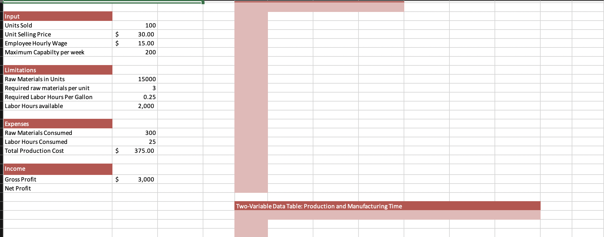
2	Create appropriate range names for Total Production Cost (cell B18) and Gross Profit (cell B21) by selection, using the values in the left column.	3
3	Edit the existing name range Employee_Hourly_Wage to Hourly_Wages2021. Note, Mac users, in the Define Name dialog box, add the new named range, and delete the original one.	3
4	Use the newly created range names to create a formula to calculate Net Profit (in cell B22). Net Profit = Gross Profit - Total Production Cost.	4
5	Create a new worksheet labeled Range Names, paste the newly created range name information in cell A1, and resize the columns as needed for proper display. Ensure that the data is sorted by range name, column A.	5
6	On the Forecast sheet, start in cell E3. Complete the series of substitution values ranging from 10 to 200 at increments of 10 gallons vertically down column E.	2
7	Enter references to the Total_Production_Cost, Gross_Profit, and Net Profit cells in the correct locations (F2, G2, and H2 respectively) for a one-variable data table. Use range names where indicated.	3
8	Complete the one-variable data table in the range E2:H22 using cell B4 as the column input cell, and then format the results with Accounting Number Format with two decimal places.	5
9	Apply custom number formats to make the formula references appear as descriptive column headings. In F2, Total Costs; in G2, Gross Profit, in H2, Net Profit. Bold and center the headings and substitution values.	3
10	Copy the number of gallons produced substitution values from the one-variable data table, and then paste the values starting in cell E26.	4
11	Type $15 in cell F25. Complete the series of substitution values from $15 to $40 at $5 increments.	4
12	Enter the reference to the net profit formula in the correct location for a two-variable data table.	4
13	Complete the two-variable data table in the range E25:K45. Use cell B6 as the Row input cell and B4 as the Column input cell. Format the results with Accounting Number Format with two decimal places.	10
14	Apply a custom number format to make the formula reference appear as a descriptive column heading Wages. Bold and center the headings and substitution values where necessary.	3
15	Create a scenario named Best Case, using Units Sold, Unit Selling Price, and Employee Hourly Wage (use cell references). Enter these values for the scenario: 200, 30, and 15.	4
16	Create a second scenario named Worst Case, using the same changing cells. Enter these values for the scenario: 100, 25, and 20.	4
17	Create a third scenario named Most Likely, using the same changing cells. Enter these values for the scenario: 150, 25, and 15.	4
18	Generate a scenario summary report using the cell references for Total Production Cost and Net Profit.	5
19	Load the Solver add-in if it is not already loaded. Set the objective to calculate the highest Net Profit possible.	5
20	Use the units sold as changing variable cells.	4
21	Use the Limitations section of the spreadsheet model to set a constraint for raw materials (The raw materials consumed must be less than or equal to the raw materials available). Use cell references to set constraints.	4
22	Set a constraint for labor hours. Use cell references to set constraints.	4
23	Set a constraint for maximum production capability. Units sold (B4) must be less than or equal to maximum capability per week (B7). Use cell references to set constraints.	4
24	Solve the problem. Generate the Answer Report and Keep Solver Solution.	5
25	Create a footer on all four worksheets with your name on the left side, the sheet name code in the center, and the file name code on the right side.	4
26	Save and close Exp19_Excel_Ch06_Cap_DeltaPaint.xlsx. Exit Excel. Submit the file as directed.	0

Total Points

100

please do the Excel!

Two-Va