t	T
0	846.22472
0.125	845.74759
0.25	845.24428
0.375	844.80459
0.5	844.34713
0.625	843.97002
0.75	843.56203
0.875	843.09525
1	842.40362
1.125	841.46356
1.25	840.23173
1.375	838.69932
1.5	836.88729
1.625	834.84218
1.75	832.59273
1.875	830.17814
2	827.62736
2.125	824.96796
2.25	822.22499
2.375	819.40985
2.5	816.54828
2.625	813.64221
2.75	810.71292
2.875	807.75079
3	804.78355
3.125	801.80949
3.25	798.83339
3.375	795.86246
3.5	792.91118
3.625	789.95597
3.75	787.02348
3.875	784.11713
4	781.22565
4.125	778.34974
4.25	775.51435
4.375	772.69965
4.5	769.9183
4.625	767.15774
4.75	764.43911
4.875	761.75176
5	759.08547
5.125	756.46262
5.25	753.86529
5.375	751.29373
5.5	748.75182
5.625	746.2446
5.75	743.77876
5.875	741.32892
6	738.90302
6.125	736.50148
6.25	734.11259
6.375	731.73361
6.5	729.3569
6.625	726.97588
6.75	724.57464
6.875	722.12623
7	719.59628
7.125	716.98178
7.25	714.20446
7.375	711.2152
7.5	707.94608
7.625	704.28738
7.75	700.13166
7.875	695.40674
8	690.0294
8.125	683.98965

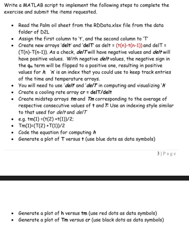
This modeling problem involves the estimation of the Heat Transfer coefficient in a quenching experiment simulation with the aid of MATLAB. You are required to compute the estimated heat transfer coefficient (h) data for an Inconel thermocouple mounted at the center face of a cylindrical probe. The hot probe is dunked into a quench tank containing different quench media at a room temperature of Ts, then the measured temperature Tm is recorded over time and this information is stored in a large EXCEL file. For this modeling exercise, download an EXCEL file RDData.xlsx from D2L, you will be using data from a sheet called Palm oil. Key data for the probe: Material: Inconel Density () = 8495 kg/m2 Diameter = 15 mm Length = 50 mm Specific heat capacity (cp) = 4198 J/kg C Temperature of the Palm oil in the quench tank is Ts = 25 C Important relationships to incorporate in your computations Heat lost by the probe = ga = h* A*(Tm-Ts) Decrease in internal energy of the probe = m = - p*V*cp*cr Under equilibrium conditions QA = 9m. Solve for h as a function of the midstep temperature, Tm Where: h = heat transfer coefficient cr = the cooling rate A = the surface area of the probe. V = volume of the probe Write a MATLAB script to implement the following steps to complete the exercise and submit the items requested. Read the Palm oil sheet from the RDData.xlsx file from the data folder of D2L Assign the first column to 't', and the second column to 'T Create new arrays 'delt' and 'delt as delt = (t(n)-1(n-1)) and delt = (T(n)-T(n-1)). As a check, delt will have negative values and delt will have positive values. With negative delt values, the negative sign in the am term will be flipped to a positive one, resulting in positive values for h. 'n' is an index that you could use to keep track entries of the time and temperature arrays. You will need to use 'delt and delt in computing and visualizing 'H Create a cooling rate array cr = delt/delt Create midstep arrays tm and Tm corresponding to the average of respective consecutive values of t and T: Use an indexing style similar to that used for delt and delt . e.g. tm(1) =(+(2) +t(1))/2; Tm(1)=(T(2) +T(1))/2 Code the equation for computing h Generate a plot of T versus (use blue dots as data symbols) 3 | Page Generate a plot of h versus tm (use red dots as data symbols) Generate a plot of Tm versus cr (use black dots as data symbols) This modeling problem involves the estimation of the Heat Transfer coefficient in a quenching experiment simulation with the aid of MATLAB. You are required to compute the estimated heat transfer coefficient (h) data for an Inconel thermocouple mounted at the center face of a cylindrical probe. The hot probe is dunked into a quench tank containing different quench media at a room temperature of Ts, then the measured temperature Tm is recorded over time and this information is stored in a large EXCEL file. For this modeling exercise, download an EXCEL file RDData.xlsx from D2L, you will be using data from a sheet called Palm oil. Key data for the probe: Material: Inconel Density () = 8495 kg/m2 Diameter = 15 mm Length = 50 mm Specific heat capacity (cp) = 4198 J/kg C Temperature of the Palm oil in the quench tank is Ts = 25 C Important relationships to incorporate in your computations Heat lost by the probe = ga = h* A*(Tm-Ts) Decrease in internal energy of the probe = m = - p*V*cp*cr Under equilibrium conditions QA = 9m. Solve for h as a function of the midstep temperature, Tm Where: h = heat transfer coefficient cr = the cooling rate A = the surface area of the probe. V = volume of the probe Write a MATLAB script to implement the following steps to complete the exercise and submit the items requested. Read the Palm oil sheet from the RDData.xlsx file from the data folder of D2L Assign the first column to 't', and the second column to 'T Create new arrays 'delt' and 'delt as delt = (t(n)-1(n-1)) and delt = (T(n)-T(n-1)). As a check, delt will have negative values and delt will have positive values. With negative delt values, the negative sign in the am term will be flipped to a positive one, resulting in positive values for h. 'n' is an index that you could use to keep track entries of the time and temperature arrays. You will need to use 'delt and delt in computing and visualizing 'H Create a cooling rate array cr = delt/delt Create midstep arrays tm and Tm corresponding to the average of respective consecutive values of t and T: Use an indexing style similar to that used for delt and delt . e.g. tm(1) =(+(2) +t(1))/2; Tm(1)=(T(2) +T(1))/2 Code the equation for computing h Generate a plot of T versus (use blue dots as data symbols) 3 | Page Generate a plot of h versus tm (use red dots as data symbols) Generate a plot of Tm versus cr (use black dots as data symbols)