

Question: Tahoma l U.shg , . ||| Quick Change Editing 2 Paragraplh Styles Styles Font Stylesr 2 Click the Places sheet tab, convert the data to
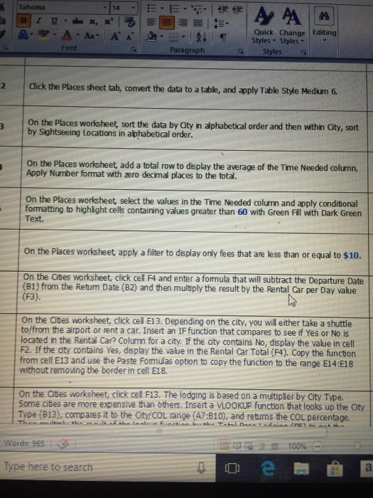
Tahoma l U.shg , . ||| Quick Change Editing 2 Paragraplh Styles Styles" Font Stylesr 2 Click the Places sheet tab, convert the data to a table, and apply Table Style Medun 6. by Sightseeing Locations in aphabetical order. On the Places worksheet, add a total row to display the average of the Time Needed column. Apply Number format with zero decimal places to the total. On the Places worksheet, select the values in the Time Needed column and apply conditional formatting to highight cells containing values greater than 60 with Green Fill with Dark Green Text. On the Places worksheet apply a filter to display only fees that are less than or equal to $10. On the Cities worksheet, click cel F4 and enter a formula that will subtract the Departure Date (B1) from the Retun Date (82) and then mulbply the result by the Rental Car per Day value (F3). On the Cites worksheet, click cell E13. Depending on the city, you will either take a shuttle to/from the airport or rent a car. Insert an IF function that compares to see if Yes or No is located in the Rental Car? Column for a city. If the aty contains No, display the value in cell F2. If the aty contains Yes, display the value in the Rental Car Total (F4). Copy the function from cell E13 and use the Paste Fomulas option to copy the function to the range E14:E18 without remoing the border in cell E18 On the Cites worksheet, click cel F13. The lodging is based on a multiplier by City Type. Some cites are more expensive than others. Insert a VLOOKUP function that looks up the City Type (813), compares it to the City/COL range (A7:B10), and retuns the COL percentage. Words: 965 3 Type here to search Tahoma l U.shg , . ||| Quick Change Editing 2 Paragraplh Styles Styles" Font Stylesr 2 Click the Places sheet tab, convert the data to a table, and apply Table Style Medun 6. by Sightseeing Locations in aphabetical order. On the Places worksheet, add a total row to display the average of the Time Needed column. Apply Number format with zero decimal places to the total. On the Places worksheet, select the values in the Time Needed column and apply conditional formatting to highight cells containing values greater than 60 with Green Fill with Dark Green Text. On the Places worksheet apply a filter to display only fees that are less than or equal to $10. On the Cities worksheet, click cel F4 and enter a formula that will subtract the Departure Date (B1) from the Retun Date (82) and then mulbply the result by the Rental Car per Day value (F3). On the Cites worksheet, click cell E13. Depending on the city, you will either take a shuttle to/from the airport or rent a car. Insert an IF function that compares to see if Yes or No is located in the Rental Car? Column for a city. If the aty contains No, display the value in cell F2. If the aty contains Yes, display the value in the Rental Car Total (F4). Copy the function from cell E13 and use the Paste Fomulas option to copy the function to the range E14:E18 without remoing the border in cell E18 On the Cites worksheet, click cel F13. The lodging is based on a multiplier by City Type. Some cites are more expensive than others. Insert a VLOOKUP function that looks up the City Type (813), compares it to the City/COL range (A7:B10), and retuns the COL percentage. Words: 965 3 Type here to search
Step by Step Solution
There are 3 Steps involved in it

Get step-by-step solutions from verified subject matter experts