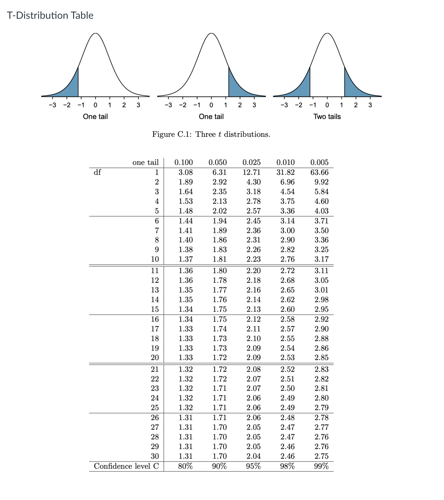
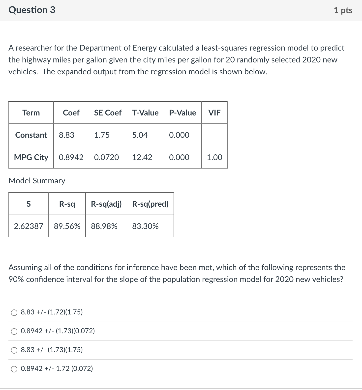
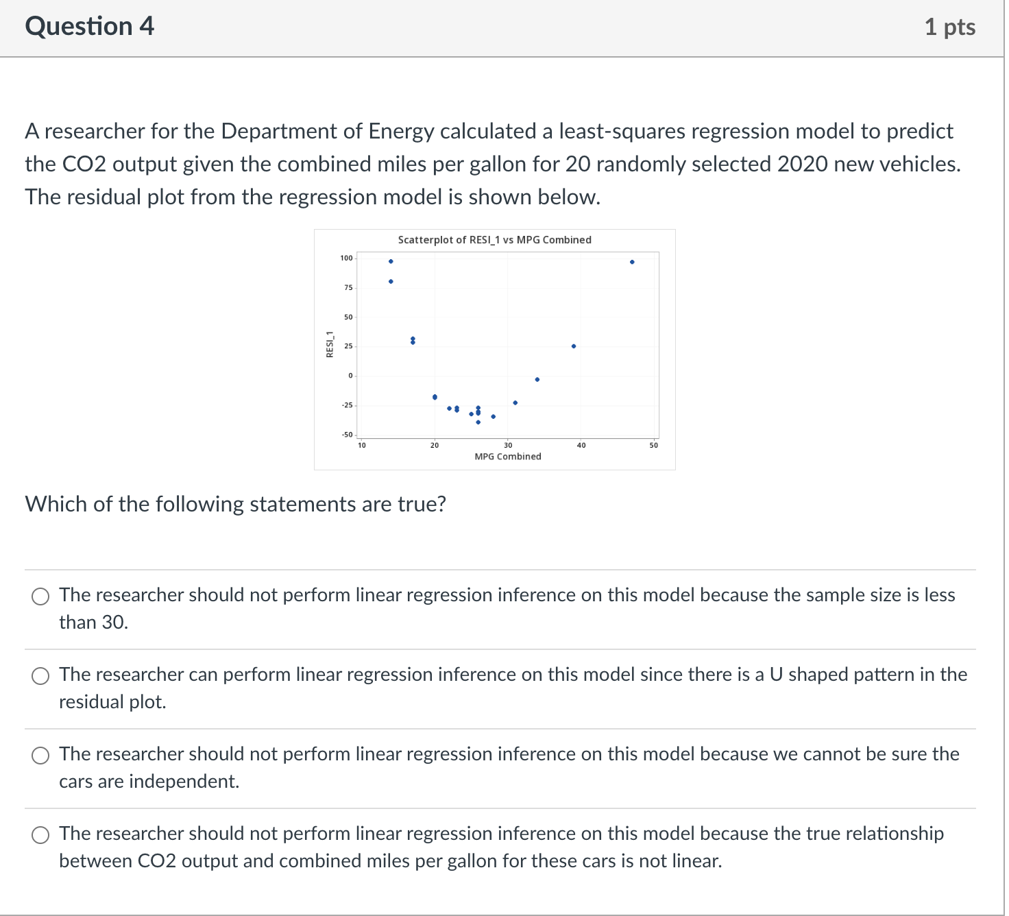
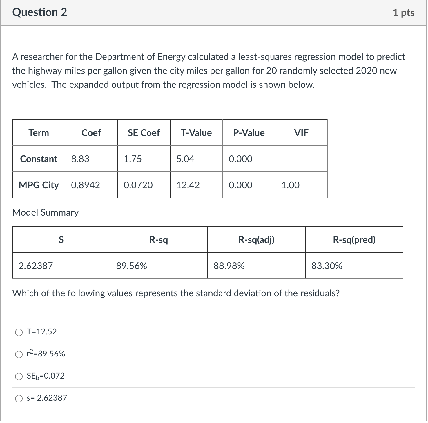
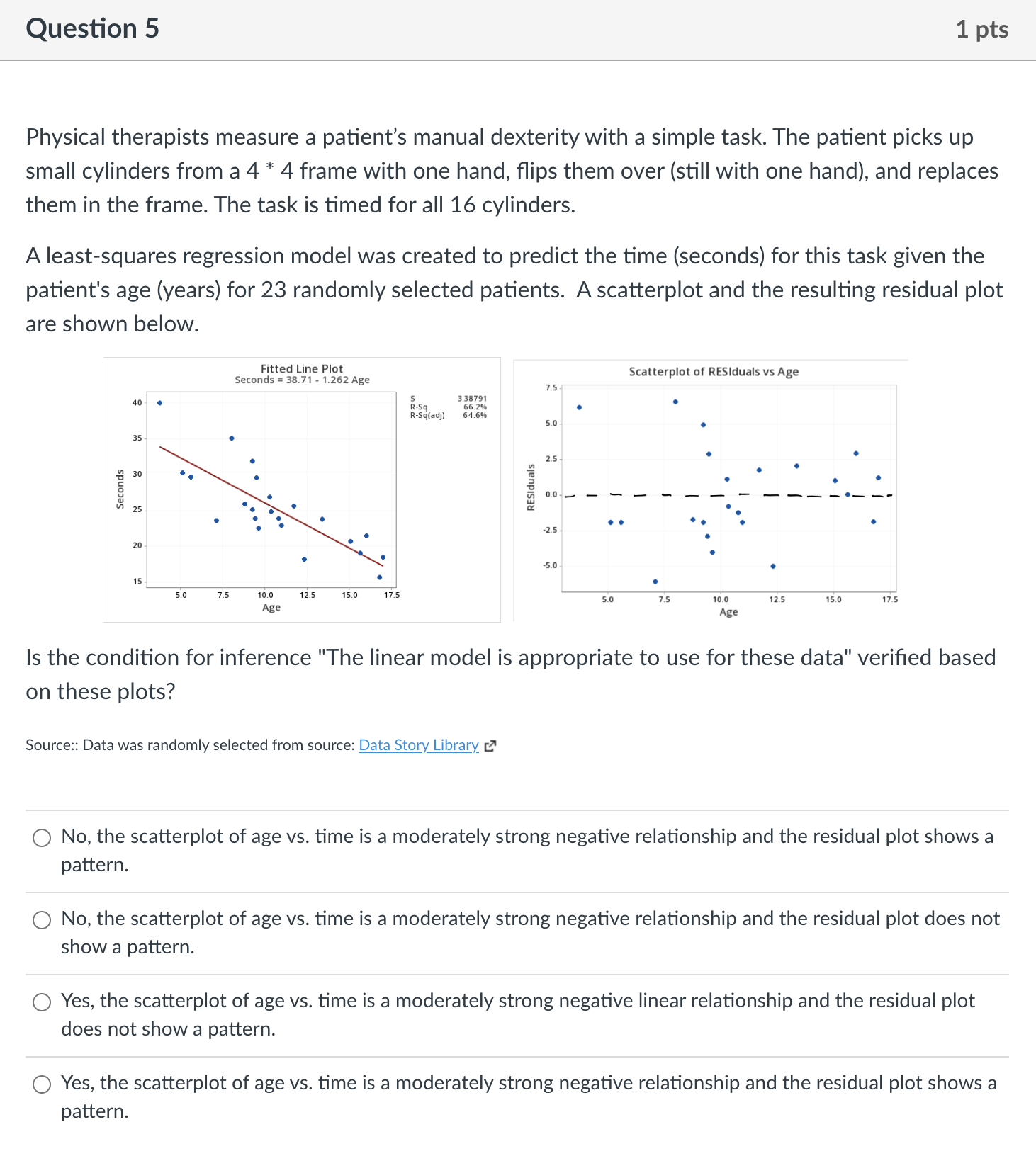
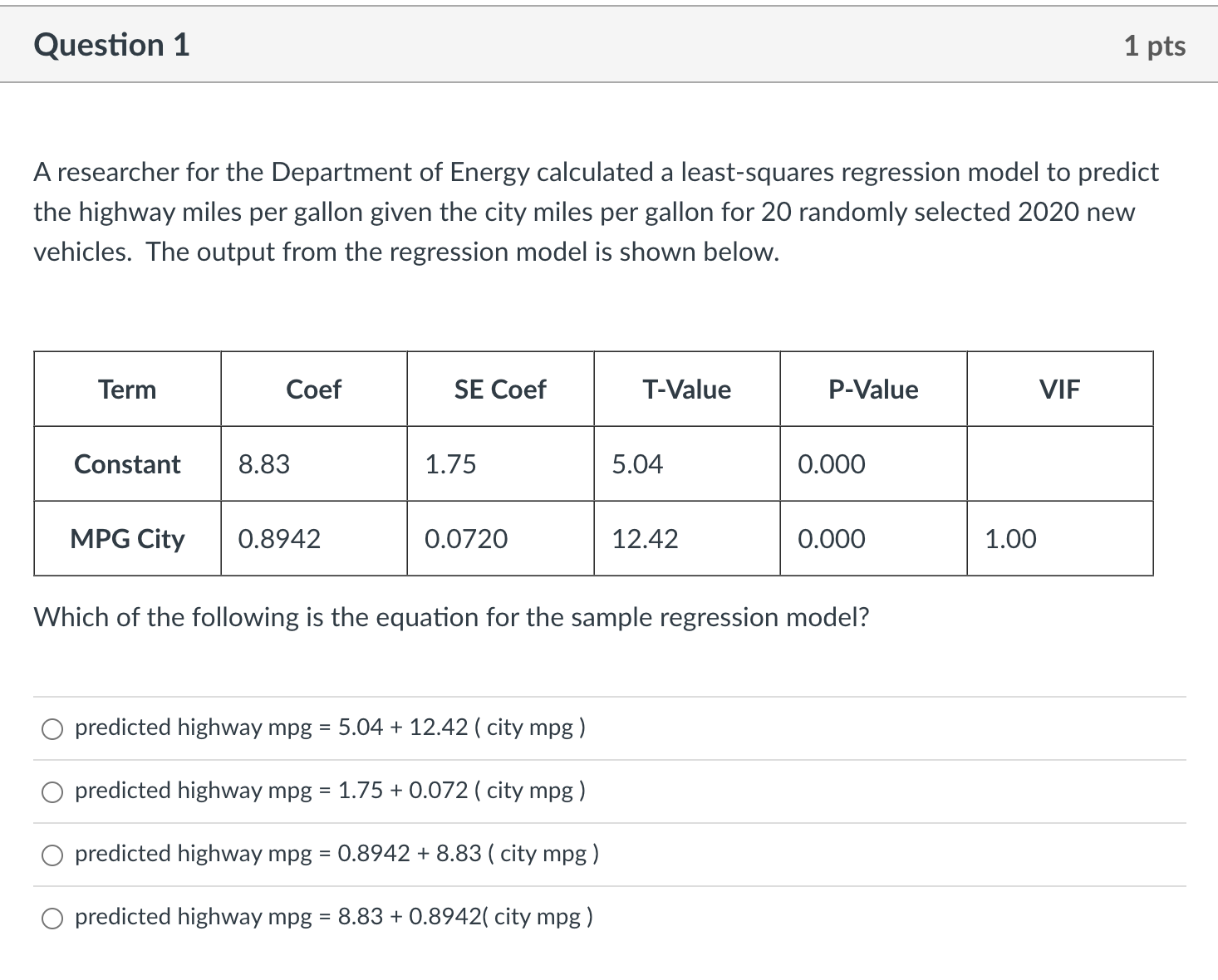
T-Distribution Table -3 -2 -1 -3 -2 -1 0 One tail One tail Two tails Figure C.1: Three t distributions. one tail 0.100 0.050 0.025 0.010 0.005 df 3.08 6.31 12.7 31.82 63.66 1.89 2.92 4.30 6.96 9.92 1.64 2.35 3.18 4.54 5.84 1.53 2.13 2.78 3.75 4.60 1.48 2.02 2.57 4.03 1.44 1.94 2.45 3.14 3.71 1.41 1.89 2.36 3.00 3.50 1.40 1.86 2.31 2.90 3.36 1.38 1.83 2.26 2.82 3.25 1.37 1.81 2.23 2.76 3.17 11 1.36 1.80 2.20 2.72 3.11 12 1.36 1.78 2.18 2.68 3.05 13 1.35 1.77 2.16 2.65 3.01 14 1.35 1.76 2.14 2.62 2.98 15 1.34 1.75 2.60 2.95 16 1.34 1.75 2.12 2.58 2.92 17 1.33 1.74 2.11 2.57 2.90 18 1.33 1.73 2.10 2.55 2.88 19 1.33 1.73 2.09 2.54 2.86 20 1.33 1.72 2.09 2.53 2.85 21 1.32 1.72 2.08 2.52 2.83 22 1.32 1.72 2.07 2.51 2.82 23 1.32 1.71 2.07 2.50 2.81 24 1.32 1.71 2.06 2.49 2.80 25 1.32 1.71 2.06 2.49 2.79 26 1.31 1.71 2.06 2.48 2.78 27 1.31 1.70 2.05 2.47 2.77 28 1.31 1.70 2.05 2.47 2.76 29 1.31 1.70 2.05 2.46 2.76 30 1.3 1.70 2.04 2.46 2.75 Confidence level C 80% 90% 95% 98% 99%Question 1 1 pts A researcher for the Department of Energy calculated a least-squares regression model to predict the highway miles per gallon given the city miles per gallon for 20 randomly selected 2020 new vehicles. The output from the regression model is shown below. MPG City 0.8942 0.0720 12.42 0.000 Which of the following is the equation for the sample regression model? O predicted highway mpg = 5.04 + 12.42 (city mpg ) O predicted highway mpg = 1.75 + 0.072 ( city mpg ) O predicted highway mpg = 0.8942 + 8.83 ( city mpg) O predicted highway mpg = 8.83 + 0.8942( city mpg) Question 2 1 pts A researcher for the Department of Energy calculated a least-squares regression model to predict the highway miles per gallon given the city miles per gallon for 20 randomly selected 2020 new vehicles. The expanded output from the regression model is shown below. MPG City 0.8942 0.0720 12.42 0.000 Model Summary 2.62387 89.56% 88.98% 83.30% Which of the following values represents the standard deviation of the residuals? O T=12.52 o r2=89.56% O SEb=0.072 O 5: 2.62387 Question 3 1 pts A researcher for the Department of Energy calculated a least-squares regression model to predict the highway miles per gallon given the city miles per gallon for 20 randomly selected 2020 new vehicles. The expanded output from the regression model is shown below. 8.83 1.75 5.04 0.000 - MPG City 0.8942 0.0720 12.42 0.000 Model Summary 2.62387 89.56% 88.98% 83.30% Assuming all of the conditions for inference have been met, which of the following represents the 90% condence interval for the slope of the population regression model for 2020 new vehicles? 0 8.83 +/- (1.72)(1.75) 0 0.8942 +/- (1.73)(0.072) O 8.83 +/- (1.73)(1.75) 0 0.8942 +/- 1.72 (0.072) Question 4 1 pts A researcher for the Department of Energy calculated a least-squares regression model to predict the C02 output given the combined miles per gallon for 20 randomly selected 2020 new vehicles. The residual plot from the regression model is shown below. Scatterplot of RES|_1vs MPG Combined 1on , o o 757 50 25- RESI_1 25 . ' '3 .3 0 0 O .5\" . In 20 so 40 so MPG Combined Which of the following statements are true? 0 The researcher should not perform linear regression inference on this model because the sample size is less than 30. O The researcher can perform linear regression inference on this model since there is a U shaped pattern in the residual plot. 0 The researcher should not perform linear regression inference on this model because we cannot be sure the cars are independent. 0 The researcher should not perform linear regression inference on this model because the true relationship between C02 output and combined miles per gallon for these cars is not linear. Question 5 1 pts Physical therapists measure a patient's manual dexterity with a simple task. The patient picks up small cylinders from a 4 * 4 frame with one hand, ips them over (still with one hand), and replaces them in the frame. The task is timed for all 16 cylinders. A least-squares regression model was created to predict the time (seconds) for this task given the patient's age (years) for 23 randomly selected patients. A scatterplot and the resulting residual plot are shown below. Fitted Line Plot Seconds = 38.71 _ 1262 Age 15. Scatterplot of RESlduals vs Age 5 3.3!791 . R-Sq an 29: - RVSqtadj} 54 596 40 I 5.07 I 35 2.5- 307 00'...___ -__-___O__- Seconds RESlduals 25. .15. 20 5.0 0 l5 . 0 5|] 7.5 100 12.5 15\" '15 Age 5.0 7 5 I03 12.5 150 \".5 Age Is the condition for inference "The linear model is appropriate to use for these data" veried based on these plots? Source: Data was randomly selected from source: Data Story Library E] O No, the scatterplot of age vs. time is a moderately strong negative relationship and the residual plot shows a pattern. 0 No, the scatterplot of age vs. time is a moderately strong negative relationship and the residual plot does not show a pattern. 0 Yes, the scatterplot of age vs. time is a moderately strong negative linear relationship and the residual plot does not show a pattern. 0 Yes, the scatterplot of age vs. time is a moderately strong negative relationship and the residual plot shows a pattern