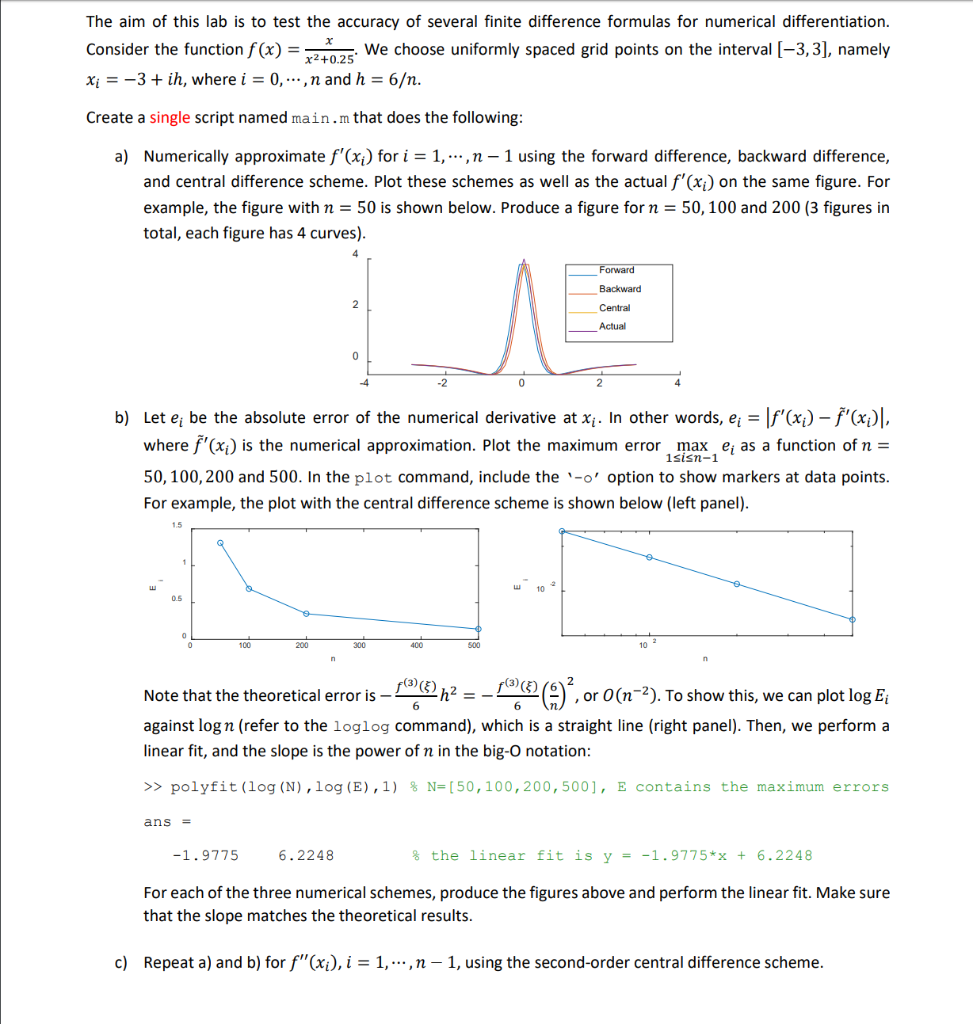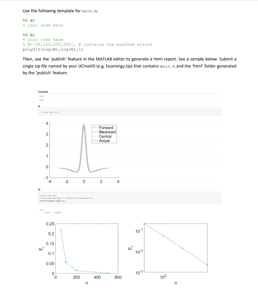
The aim of this lab is to test the accuracy of several finite difference formulas for numerical differentiation. Consider the function f(x) = 2:02 We choose uniformly spaced grid points on the interval (-3,3), namely Xi = -3 + ih, where i = 0,...,n and h = 6. Create a single script named main.m that does the following: a) Numerically approximate f'(xi) for i = 1,...,n - 1 using the forward difference, backward difference, and central difference scheme. Plot these schemes as well as the actual f'(xi) on the same figure. For example, the figure with n = 50 is shown below. Produce a figure for n = 50, 100 and 200 (3 figures in total, each figure has 4 curves). Forward Backward Central Actual 0 b) Let e; be the absolute error of the numerical derivative at xi. In other words, e; = f'(xi) - f'(x), where f'(xi) is the numerical approximation. Plot the maximum error max ei as a function of n = isisn-1 50, 100, 200 and 500. In the plot command, include the '-o' option to show markers at data points. For example, the plot with the central difference scheme is shown below (left panel). w 10 100 200 300 400 500 Note that the theoretical error is 9h2 = -102 )', or 0(n=2). To show this, we can plot log E; against log n (refer to the loglog command), which is a straight line (right panel). Then, we perform a linear fit, and the slope is the power of n in the big-O notation: >> polyfit(log (N), log (E),1) % N=[50, 100, 200,500], E contains the maximum errors ans = -1.97756.2248 % the linear fit is y = -1.9775*x + 6.2248 For each of the three numerical schemes, produce the figures above and perform the linear fit. Make sure that the slope matches the theoretical results. c) Repeat a) and b) for F"(xi), i = 1,..., n-1, using the second-order central difference scheme. Use the following template for main.m. f your code here %% b) % your code here % N=[50, 100, 200, 500], E contains the maximum errors polyfit(log (N), log (E),1) Then, use the "publish' feature in the MATLAB editor to generate a html report. See a sample below. Submit a single zip file named by your UCInetID (e.g. huamingy.zip) that contains main.m and the 'html' folder generated by the 'publish' feature. Contents $ your code here Forward Backward Central - Actual 4 -2 0 2 4 your code here SMS, 100, 200, 500). E contains the main errors polyfit(log().log(),1) 1.97756 .2248 0.25 0.2 10-1 w 0.1 0.05 0 200 400 600 1 103 102 The aim of this lab is to test the accuracy of several finite difference formulas for numerical differentiation. Consider the function f(x) = 2:02 We choose uniformly spaced grid points on the interval (-3,3), namely Xi = -3 + ih, where i = 0,...,n and h = 6. Create a single script named main.m that does the following: a) Numerically approximate f'(xi) for i = 1,...,n - 1 using the forward difference, backward difference, and central difference scheme. Plot these schemes as well as the actual f'(xi) on the same figure. For example, the figure with n = 50 is shown below. Produce a figure for n = 50, 100 and 200 (3 figures in total, each figure has 4 curves). Forward Backward Central Actual 0 b) Let e; be the absolute error of the numerical derivative at xi. In other words, e; = f'(xi) - f'(x), where f'(xi) is the numerical approximation. Plot the maximum error max ei as a function of n = isisn-1 50, 100, 200 and 500. In the plot command, include the '-o' option to show markers at data points. For example, the plot with the central difference scheme is shown below (left panel). w 10 100 200 300 400 500 Note that the theoretical error is 9h2 = -102 )', or 0(n=2). To show this, we can plot log E; against log n (refer to the loglog command), which is a straight line (right panel). Then, we perform a linear fit, and the slope is the power of n in the big-O notation: >> polyfit(log (N), log (E),1) % N=[50, 100, 200,500], E contains the maximum errors ans = -1.97756.2248 % the linear fit is y = -1.9775*x + 6.2248 For each of the three numerical schemes, produce the figures above and perform the linear fit. Make sure that the slope matches the theoretical results. c) Repeat a) and b) for F"(xi), i = 1,..., n-1, using the second-order central difference scheme. Use the following template for main.m. f your code here %% b) % your code here % N=[50, 100, 200, 500], E contains the maximum errors polyfit(log (N), log (E),1) Then, use the "publish' feature in the MATLAB editor to generate a html report. See a sample below. Submit a single zip file named by your UCInetID (e.g. huamingy.zip) that contains main.m and the 'html' folder generated by the 'publish' feature. Contents $ your code here Forward Backward Central - Actual 4 -2 0 2 4 your code here SMS, 100, 200, 500). E contains the main errors polyfit(log().log(),1) 1.97756 .2248 0.25 0.2 10-1 w 0.1 0.05 0 200 400 600 1 103 102