

Answered step by step
Verified Expert Solution
Question
1 Approved Answer
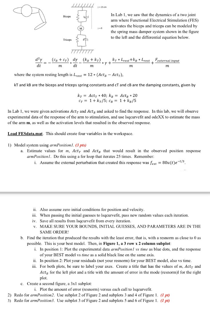
The biceps and triceps can be modeled by the spring mass damper system shown in the figure to the left and the differential equation below.
The biceps and triceps can be modeled by
the spring mass damper system shown in the figure
to the left and the differential equation below.
where the system resting length is
and are the biceps and triceps spring constants and and are the damping constants, given by
;
;
We were previosusly given activations and and asked to find the response. In this lab, we will observe
experimental data of the response of the arm to stimulation, and use lsqcurvefit and odeXX to estimate the mass
of the arm as well as the activation levels that resulted in the observed response.
In MATLAB: Load FESdata.mat. This should create four variables in the workspace.
Model system using armPosition pts
a Estimate values for and that would result in the observed position response
armPositionI. Do this using a for loop that iterates times. Remember:
i Assume the external perturbation that created this response was
ii Also assume zero initial conditions for position and velocity.
iii. When passing the initial guesses to lsqcurvefit, pass new random values each iteration.
iv Save all results from Isqcurvefit from every iteration.
v MAKE SURE YOUR BOUNDS, INITIAL GUESSES, AND PARAMETERS ARE IN THE
SAME ORDER!
b Find the iteration that produced the results with the least error, that is with a resnorm as close to as
possible. This is your best model. Then, in Figure a row column subplot:
i In position : Plot the experimental data armPosition I vs time as blue dots, and the response
of your BEST model vs time as a solid black line on the same axis.
ii In position : Plot your residuals not your resnorm for your BEST model, also vs time.
iii. For both plots, be sure to label your axes. Create a title that has the values of and
for the left plot and a title with the amount of error in the mode resnorml for the right
plot.
c Create a second figure, a subplot:
i Plot the amount of error resnorm versus each call to lsqcurvefit.
Redo for armPosition Use subplot of Figure and subplots and of Figure
Redo for armPosition Use subplot of Figure and subplots and of Figure pt
Step by Step Solution
There are 3 Steps involved in it
Step: 1

Get Instant Access to Expert-Tailored Solutions
See step-by-step solutions with expert insights and AI powered tools for academic success
Step: 2

Step: 3
Ace Your Homework with AI
Get the answers you need in no time with our AI-driven, step-by-step assistance
Get Started
Database Design Using Entity Relationship Diagrams
Authors: Sikha Saha Bagui, Richard Walsh Earp
3rd Edition
103201718X, 978-1032017181