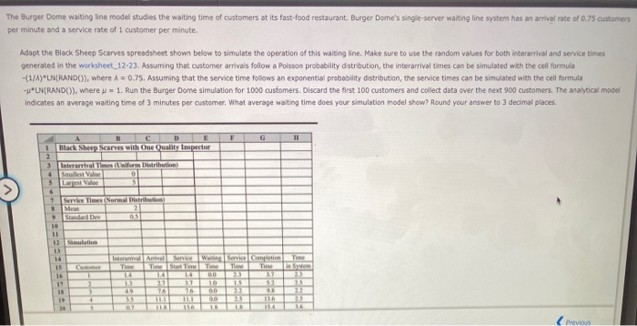
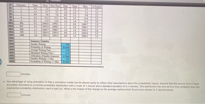
The Burger Dome waiting line model studies the waiting time of customers at its fast-food restaurant. Burger Dome's single-server waiting line system has an arrival rate of 0.75 customers per minute and a service rate of 1 customer per minute. Adapt the Black Sheep Scarves spreadsheet shown below to simulate the operation of this waiting line. Make sure to use the random values for both interarrival and service times generated in the worksheet_12-23. Assuming that customer arrivals follow a Poisson probability distribution, the interarrival times can be simulated with the cell formula -(1/A)*LN(RANDO), where 1 = 0.75. Assuming that the service time follows an exponential probability distribution, the service times can be simulated with the cell formula --*UNCRANDO), where u = 1. Run the Burger Dome simulation for 1000 customers. Discard the first 100 customers and collect data over the next 900 customers. The analytical model indicates an average waiting time of 3 minutes per customer. What average walting time does your simulation model show? Round your answer to 3 decimal places. F G H B D E Estack Sheep Scarves with One Quality Inspector 1 2 Interarrival Times wiform Distribution Smallest Value 0 4 5 6 Serie The Normal Distri Me 2 10 11 12 Mutton 13 14 15 16 Time 14 Service Service Completion Start Time Time 00 17 27 17 10 13 76 76 00 20 116 1 225 275 22 3 4 18 19 07 1 Previous Come Time in System 1 15 16 17 18 19 20 1011 Time 1.4 2.7 7.6 Sut Time 14 37 7.6 2 3 4 5 996 997 49 35 0.7 05 02 27 3.7 40 Time 00 1.0 0.0 OLO 1.8 1.3 1.7 10 0.0 0.0 136 24981 24987 25007 Time 23 15 22 25 1S 0.6 20 18 2.4 1.9 1012 Time 3.7 52 98 136 154 24987 25007 25025 2505 25093 25 22 25 316 19 3.7 28 24 19 24970 2499 7 25034 25074 1000 25074 1013 1014 1015 1016 1017 1018 1019 102 1021 1022 1023 1024 Summary Statistics Number Waiting Motability of Waiting Average Waing Time Maximum Waiting Time Uution of Quality Inspector Number Waiting > Min Probability of Waiting > Min 549 0.6100 1.59 1335 070 393 04457 minutes a. One advantage of using simulation is that a simulation model can be altered easily to reflect other assumptions about the probabilistic inputs. Assume that the service time is more accurately described by a normal probability distribution with a mean of 1 minute and a standard deviation of 0.2 minutes. This distribution has less service time variability than the exponential probability distribution used in part (a). What is the impact of this change on the average waiting time? Round your answer to 3 decimal places. minutes The Burger Dome waiting line model studies the waiting time of customers at its fast-food restaurant. Burger Dome's single-server waiting line system has an arrival rate of 0.75 customers per minute and a service rate of 1 customer per minute. Adapt the Black Sheep Scarves spreadsheet shown below to simulate the operation of this waiting line. Make sure to use the random values for both interarrival and service times generated in the worksheet_12-23. Assuming that customer arrivals follow a Poisson probability distribution, the interarrival times can be simulated with the cell formula -(1/A)*LN(RANDO), where 1 = 0.75. Assuming that the service time follows an exponential probability distribution, the service times can be simulated with the cell formula --*UNCRANDO), where u = 1. Run the Burger Dome simulation for 1000 customers. Discard the first 100 customers and collect data over the next 900 customers. The analytical model indicates an average waiting time of 3 minutes per customer. What average walting time does your simulation model show? Round your answer to 3 decimal places. F G H B D E Estack Sheep Scarves with One Quality Inspector 1 2 Interarrival Times wiform Distribution Smallest Value 0 4 5 6 Serie The Normal Distri Me 2 10 11 12 Mutton 13 14 15 16 Time 14 Service Service Completion Start Time Time 00 17 27 17 10 13 76 76 00 20 116 1 225 275 22 3 4 18 19 07 1 Previous Come Time in System 1 15 16 17 18 19 20 1011 Time 1.4 2.7 7.6 Sut Time 14 37 7.6 2 3 4 5 996 997 49 35 0.7 05 02 27 3.7 40 Time 00 1.0 0.0 OLO 1.8 1.3 1.7 10 0.0 0.0 136 24981 24987 25007 Time 23 15 22 25 1S 0.6 20 18 2.4 1.9 1012 Time 3.7 52 98 136 154 24987 25007 25025 2505 25093 25 22 25 316 19 3.7 28 24 19 24970 2499 7 25034 25074 1000 25074 1013 1014 1015 1016 1017 1018 1019 102 1021 1022 1023 1024 Summary Statistics Number Waiting Motability of Waiting Average Waing Time Maximum Waiting Time Uution of Quality Inspector Number Waiting > Min Probability of Waiting > Min 549 0.6100 1.59 1335 070 393 04457 minutes a. One advantage of using simulation is that a simulation model can be altered easily to reflect other assumptions about the probabilistic inputs. Assume that the service time is more accurately described by a normal probability distribution with a mean of 1 minute and a standard deviation of 0.2 minutes. This distribution has less service time variability than the exponential probability distribution used in part (a). What is the impact of this change on the average waiting time? Round your answer to 3 decimal places. minutes