the data set is :

"vol" "wht" "age" "bh" "pc" "aps" 0.56 15.95 50 0.25 0.25 0.65 0.37 27.65 58 0.25 0.25 0.85 0.6 14.75 74 0.25 0.25 0.85 0.3 26.65 58 0.25 0.25 0.85 2.12 30.95 62 0.25 0.25 1.45 0.35 25.25 50 0.25 0.25 2.15 2.09 32.25 64 1.85 0.25 2.15 2 34.45 58 4.65 0.25 2.35 0.46 34.45 47 0.25 0.25 2.85 1.25 25.65 63 0.25 0.25 2.85 1.29 36.75 65 0.25 0.25 3.55 3.34 31.25 57 0.25 0.65 4.05 0.66 33.65 70 3.47 0.55 4.35 0.57 26.25 41 0.25 0.25 4.75 1.2 45.85 70 5.25 0.25 4.95 3.15 30.55 59 0.25 0.25 5.15 0.58 29.25 59 0.45 0.25 5.45 5.94 31.55 63 1.55 3.25 5.55 4.25 22.75 68 1.35 0.25 5.85 1.67 41.25 65 0.25 0.45 6.05 0.67 47.75 67 6.15 0.25 6.15 2.83 22.85 67 1.25 1.05 6.35 11.13 29.25 65 0.25 5.05 6.65 1.33 59.75 65 7.12 0.45 6.85 3.58 20.85 71 3.55 0.25 7.45 1.01 26.25 54 0.25 0.25 7.55 0.99 24.95 63 0.25 0.45 7.75 3.7 61.55 64 8.77 0.25 8.05 4.15 38.75 73 0.56 5.25 8.65 1.58 10.75 64 0.25 0.25 8.95 2.22 20.35 56 2.55 0.85 9.75 1.86 23.15 60 0.25 0.25 9.95 4.23 39.75 68 0.25 0.25 10.05 1.79 47.75 62 5.55 0.65 10.25 4.42 30.25 66 5.75 0.65 12.45 15.3 54.35 79 6.55 14.25 13.05 3.2 56.55 68 5.55 0.65 13.05 5.73 33.05 43 0.25 0.25 13.35 3.39 35.45 70 3.95 0.45 13.35 2.98 54.25 68 0.25 0.25 14.25 5.26 69.05 64 7.95 0.25 14.55 1.67 37.85 64 4.45 1.05 14.65 8.39 61.65 68 5.85 4.25 14.75 23.42 33.65 59 0.25 0.25 14.95 3.55 72.25 66 8.35 0.25 15.15 2.65 17.55 47 0.25 1.65 16.25 1.59 43.15 49 4.15 0.25 16.35 1.72 65.25 70 1.55 0.25 16.55 2.89 47.05 61 3.65 0.25 16.65 1.58 92.25 73 10.24 0.25 17.15 7.37 41.25 63 5.05 6.75 17.35 16.05 33.95 72 0.25 4.75 17.35 7.65 50.25 66 7.45 8.25 17.85 7.95 37.45 64 0.25 0.25 17.85 4.3 46.35 61 3.75 0.65 17.95 7.56 48.35 68 5.95 3.75 18.55 9.01 57.45 72 10.05 0.65 19.35 0.64 82.15 69 0.25 0.25 19.35 3.19 28.25 77 5.75 0.25 20.85 3.37 45.85 69 0.25 1.25 21.25 6.29 25.45 60 1.55 3.25 21.65 20.07 46.95 69 0.25 6.75 26.45 7.47 84.25 72 8.35 1.65 29.75 12.65 77.85 78 10.24 0.25 31.05 14.13 35.95 69 0.25 13.25 31.75 16.11 45.75 63 0.25 1.45 33.55 4.34 21.55 66 1.75 1.25 33.65 13.64 48.85 77 0.59 1.75 35.35 14.55 46.45 65 3.05 5.75 35.55 4.77 40.85 60 5.45 2.25 36.15 7.57 41.75 58 5.15 0.25 39.65 5.65 29.05 62 0.25 1.35 40.95 16.57 111.95 65 0.25 11.75 53.75 25.7 60.45 68 0.25 0.25 56.25 12.59 39.55 61 3.85 0.25 62.15 16.95 48.25 68 0.25 3.75 80.25 45.65 49.25 44 0.25 8.75 108.25 18.31 29.85 52 0.25 11.75 171.25 17.86 43.55 68 4.75 4.75 239.25 32.2 53.25 68 1.55 18.25 265.85

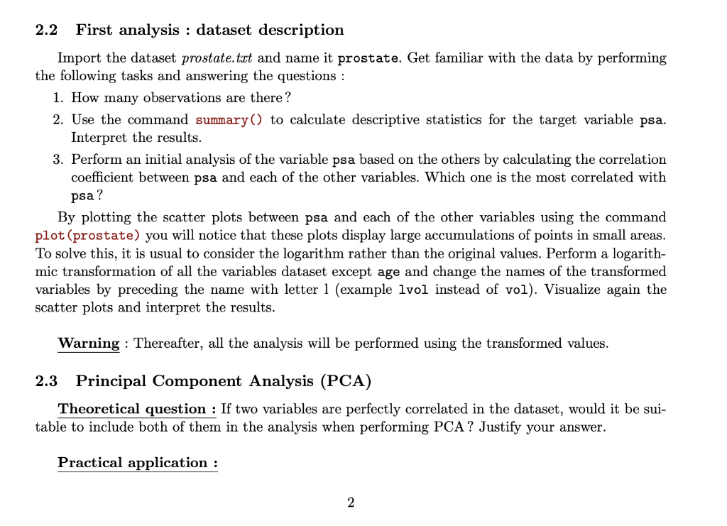
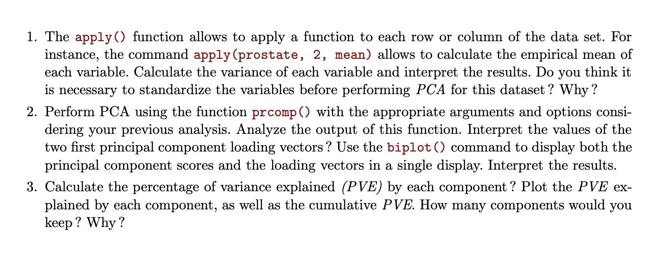
2.2 First analysis : dataset description Import the dataset prostate.tact and name it prostate. Get familiar with the data by performing the following tasks and answering the questions : 1. How many observations are there? 2. Use the command summary() to calculate descriptive statistics for the target variable psa. Interpret the results. 3. Perform an initial analysis of the variable psa based on the others by calculating the correlation coefficient between psa and each of the other variables. Which one is the most correlated with psa? By plotting the scatter plots between psa and each of the other variables using the command plot (prostate) you will notice that these plots display large accumulations of points in small areas. To solve this, it is usual to consider the logarithm rather than the original values. Perform a logarith- mic transformation of all the variables dataset except age and change the names of the transformed variables by preceding the name with letter 1 (example lvol instead of vol). Visualize again the scatter plots and interpret the results. Warning: Thereafter, all the analysis will be performed using the transformed values. 2.3 Principal Component Analysis (PCA) Theoretical question : If two variables are perfectly correlated in the dataset, would it be sui- table to include both of them in the analysis when performing PCA? Justify your answer. Practical application : 1. The apply() function allows to apply a function to each row or column of the data set. For instance, the command apply (prostate, 2, mean) allows to calculate the empirical mean of each variable. Calculate the variance of each variable and interpret the results. Do you think it is necessary to standardize the variables before performing PCA for this dataset ? Why? 2. Perform PCA using the function prcomp () with the appropriate arguments and options consi- dering your previous analysis. Analyze the output of this function. Interpret the values of the two first principal component loading vectors ? Use the biplot() command to display both the principal component scores and the loading vectors in a single display. Interpret the results. 3. Calculate the percentage of variance explained (PVE) by each component ? Plot the PVE ex- plained by each component, as well as the cumulative PVE. How many components would you keep? Why? 2.2 First analysis : dataset description Import the dataset prostate.tact and name it prostate. Get familiar with the data by performing the following tasks and answering the questions : 1. How many observations are there? 2. Use the command summary() to calculate descriptive statistics for the target variable psa. Interpret the results. 3. Perform an initial analysis of the variable psa based on the others by calculating the correlation coefficient between psa and each of the other variables. Which one is the most correlated with psa? By plotting the scatter plots between psa and each of the other variables using the command plot (prostate) you will notice that these plots display large accumulations of points in small areas. To solve this, it is usual to consider the logarithm rather than the original values. Perform a logarith- mic transformation of all the variables dataset except age and change the names of the transformed variables by preceding the name with letter 1 (example lvol instead of vol). Visualize again the scatter plots and interpret the results. Warning: Thereafter, all the analysis will be performed using the transformed values. 2.3 Principal Component Analysis (PCA) Theoretical question : If two variables are perfectly correlated in the dataset, would it be sui- table to include both of them in the analysis when performing PCA? Justify your answer. Practical application : 1. The apply() function allows to apply a function to each row or column of the data set. For instance, the command apply (prostate, 2, mean) allows to calculate the empirical mean of each variable. Calculate the variance of each variable and interpret the results. Do you think it is necessary to standardize the variables before performing PCA for this dataset ? Why? 2. Perform PCA using the function prcomp () with the appropriate arguments and options consi- dering your previous analysis. Analyze the output of this function. Interpret the values of the two first principal component loading vectors ? Use the biplot() command to display both the principal component scores and the loading vectors in a single display. Interpret the results. 3. Calculate the percentage of variance explained (PVE) by each component ? Plot the PVE ex- plained by each component, as well as the cumulative PVE. How many components would you keep? Why