The following is the template to help complete part 3 and 4:

%%% 2-D Transport: Convection + Diffusion L=1; % Length of the square N=..; % Number of nodal points discretized in the x-dir and y-dir iter=..; % number of iterations for Gauss-Seidel solver Phi_init=..; % Initial guess dx=L/(N-1); dy=L/(N-1); rho=1; % Density gamma=0.01; % Diffusion coefficient % Initialize the matrixes and vectors Phi=zeros(N,N,iter); P=zeros(N,N,3); x=zeros(N,1); y=zeros(N,1); u=zeros(N,1); v=zeros(N,1); for i=1:1:N x(i,1)=dx*(i-1); y(i,1)=dy*(i-1); end

% Initial guess of phi for the internal nodal points of the square

for i=2:1:N-1

for j=2:1:N-1

Phi(i,j,1)=Phi_init; % Initial guess in the square

end

end

% Boundary conditions

for i=1:1:N

Phi(i,1,1)=.........; % Left boundary

end

for j=2:1:N

Phi(N,j,1)=..; % Top boundary

end

for j=2:1:(N-1)

Phi(1,j,1)=..; % Bottom boundary

end

for i=1:1:(N-1)

Phi(i,N,1)=..; % Right boundary

end

% Velocity profile:

for i=1:1:N

u(i,1)=..;

v(i,1)=-..;

end

De=; Dw=; Dn=; Ds=;

%%%%%%%%%%%%%%% Deferred-correction %%%%%%%%%%%%%%%% for beta=1:1:3 B=0.25*beta; % Blending factor %%%Iterations for k=2:1:iter % Boundary conditions (left, top, and bottom) for i=1:1:N Phi(i,1,k)=..............; end for j=2:1:N Phi(N,j,k)=......................; end for j=2:1:(N-1) Phi(1,j,k)=; end % Internal nodal points for i=2:1:N-1 for j=2:1:N-1 Fe=; Fw=; Fn= ; Fs= ; % The coefficients for the first-order up-winding method aw_UW= ; ae_UW= ; an_UW= ; as_UW= ; ap_UW= ; % The coefficients for the central differencing method aw_CD= ; ae_CD= ; an_CD= ; as_CD= ; ap_CD= ; % Deferred Correction: S_DC=; Phi(i,j,k)=; end end

% Boundary conditions (right)

for i=1:1:(N-1)

Phi(i,N,k)=;

end

end

% Final results

for i=1:1:N

for j=1:1:N

P(i,j,beta)=Phi(i,j,iter);

end

end

end

% Calculate the flux through the boundary at x=0: F(1,1)=..........; Flux=F(1,1)*(dy/2); for i=2:1:N-1 F(i,1)=..........; Flux=Flux+F(i,1)*dy; end F(N,1)=..........; Flux=Flux+F(N,1)*(dy/2)

% Contour plot for the blending factor B=0.5 figure(1); .......... % Line plots along the X-X axis figure(2); dxx=sqrt(2)/(N-1); for beta=1:1:3 for i=1:1:N XX(i,1)=dxx*(i-1); P_ac(i,beta)= ..........; end end plot(XX,P_ac(:,1),'r-','LineWidth',1.5); hold on; plot(XX,P_ac(:,2),'b--','LineWidth',1.5); plot(XX,P_ac(:,3),'k+','LineWidth',1.5); hold off; xlabel('X-X Axis'); ylabel('Phi'); legend('beta=0.25','beta=0.5','beta=0.75'); grid on;

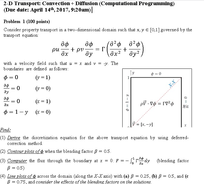
2-D Transport: Convection Diffusion (Computational Programming Due date: April 14th, 2017, 9:20am)l Problem 1 (100 points) Consider property transport in a two-dimensional domain such that x, y E 0,1 governed by the transport equation with a velocity field such that u x and v -y. The boundaries are defined as follows: ax Find (1) Derive the discretization equation for the above transport equation by using deferred correction method. (2) Contour plots when the blending factor B 0.5 30 Computer the flux through the boundary at x o: F J r dy blending factor 0.5) 4) Line plots of b across the domain (along the X- axis) with (a) B 0.25 (b) B 0.5, and (c B 0.75, and consider the effects af the blending factars an the salutians. 2-D Transport: Convection Diffusion (Computational Programming Due date: April 14th, 2017, 9:20am)l Problem 1 (100 points) Consider property transport in a two-dimensional domain such that x, y E 0,1 governed by the transport equation with a velocity field such that u x and v -y. The boundaries are defined as follows: ax Find (1) Derive the discretization equation for the above transport equation by using deferred correction method. (2) Contour plots when the blending factor B 0.5 30 Computer the flux through the boundary at x o: F J r dy blending factor 0.5) 4) Line plots of b across the domain (along the X- axis) with (a) B 0.25 (b) B 0.5, and (c B 0.75, and consider the effects af the blending factars an the salutians