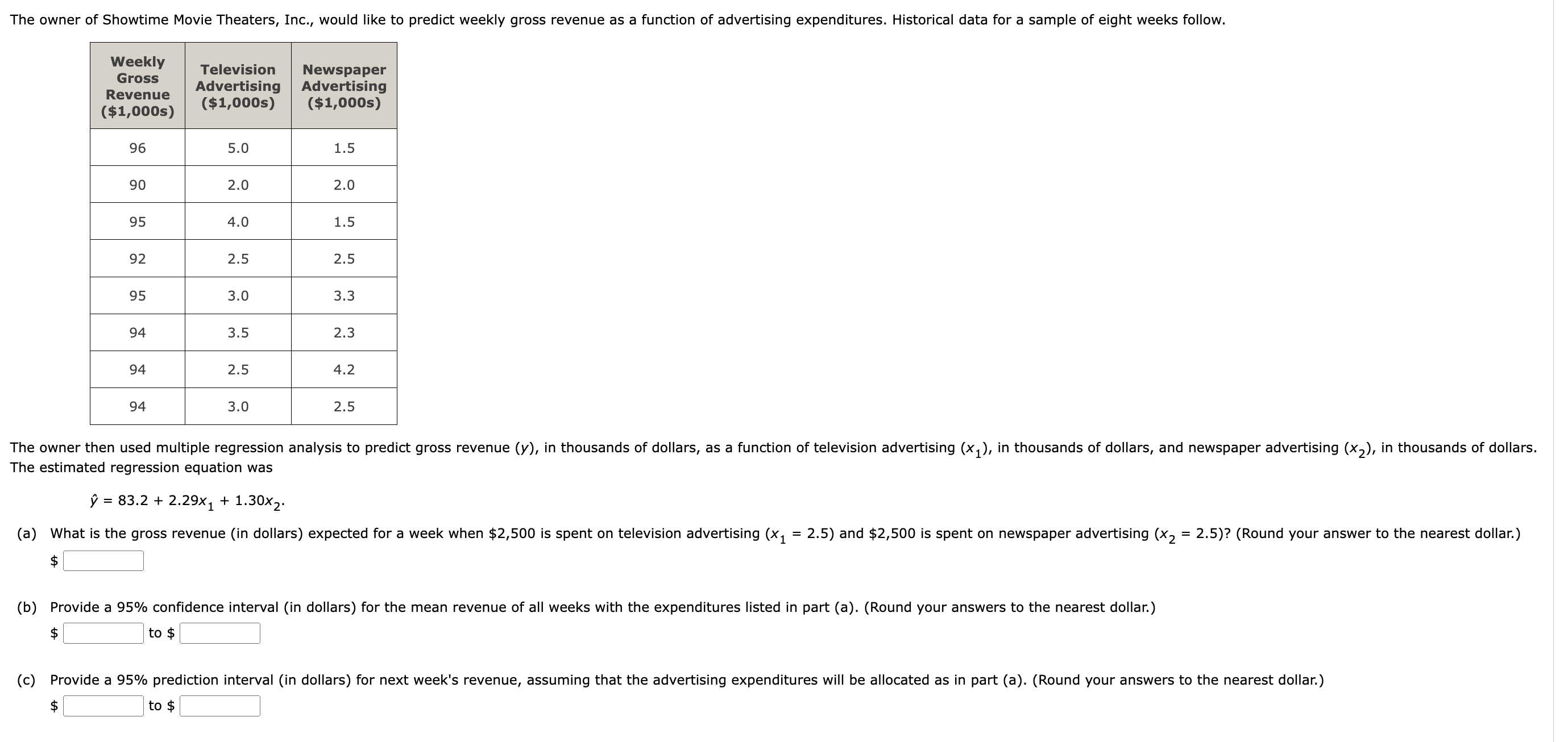
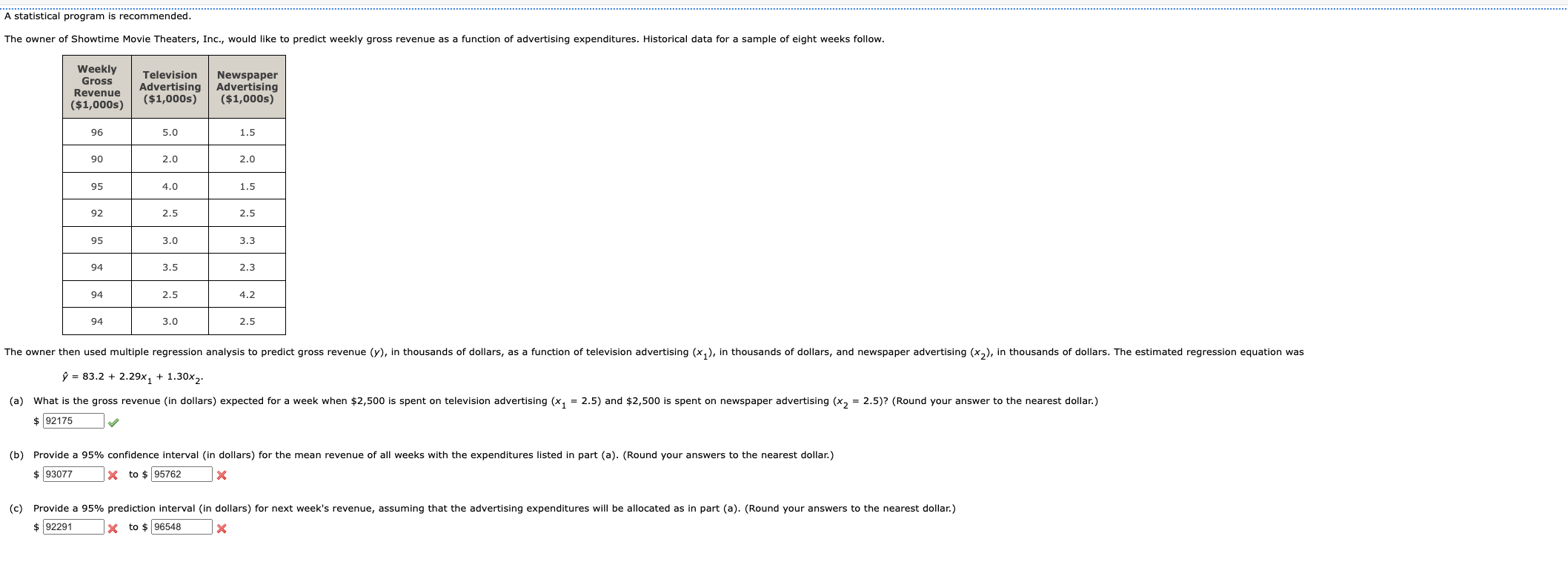
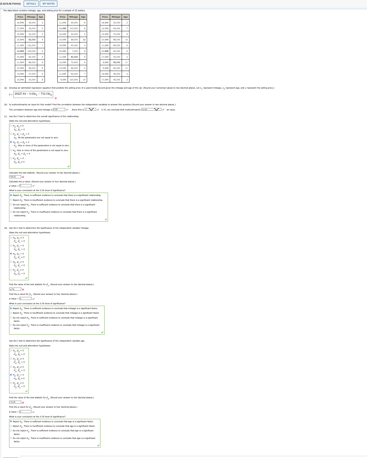
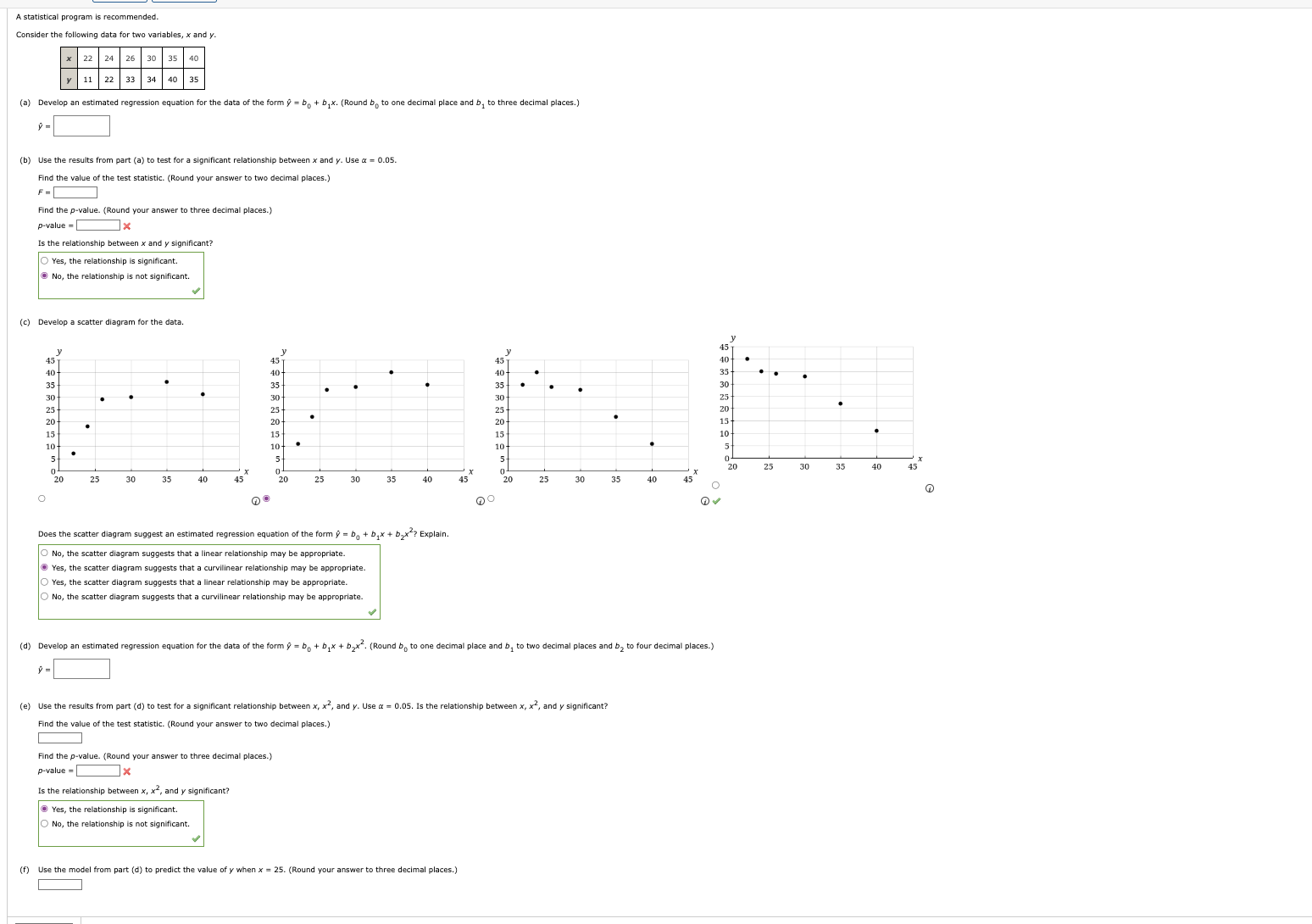
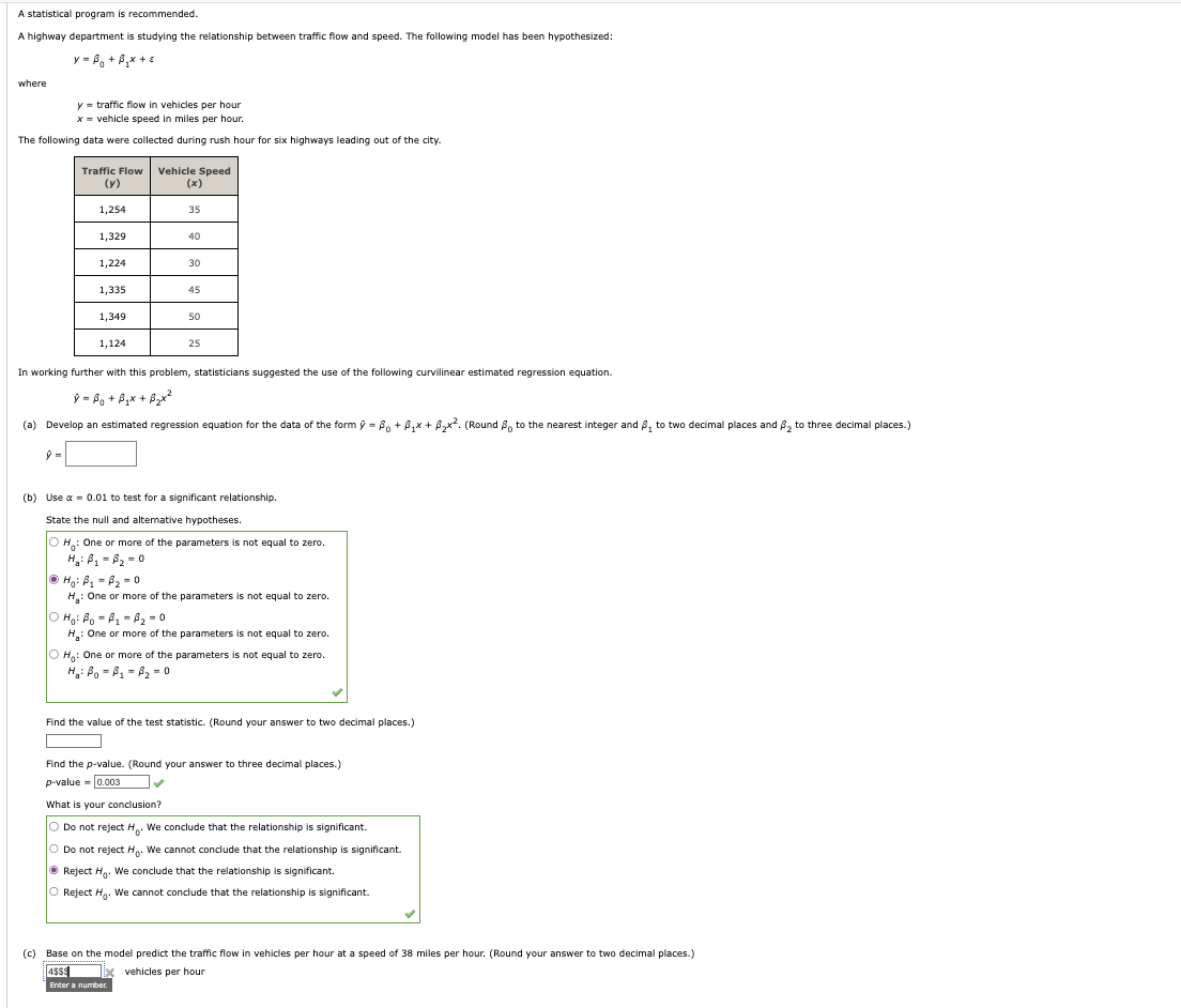
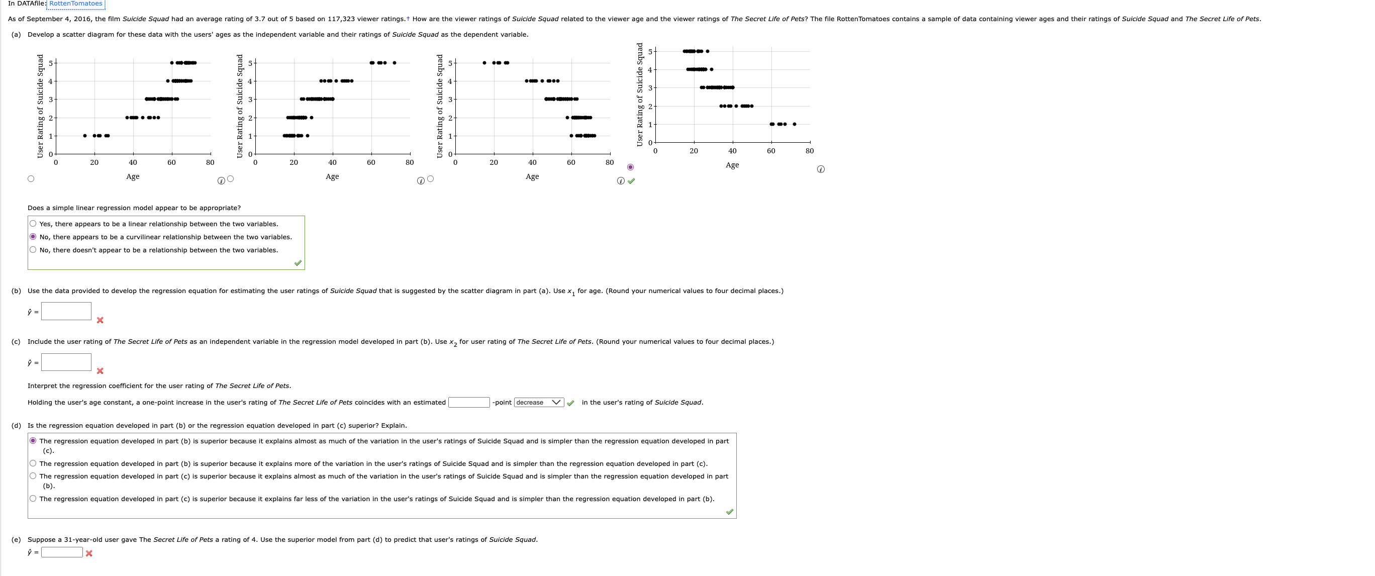
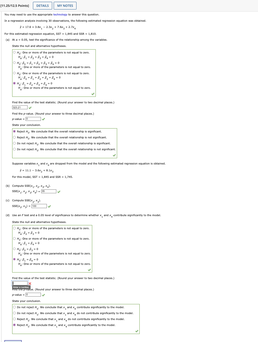
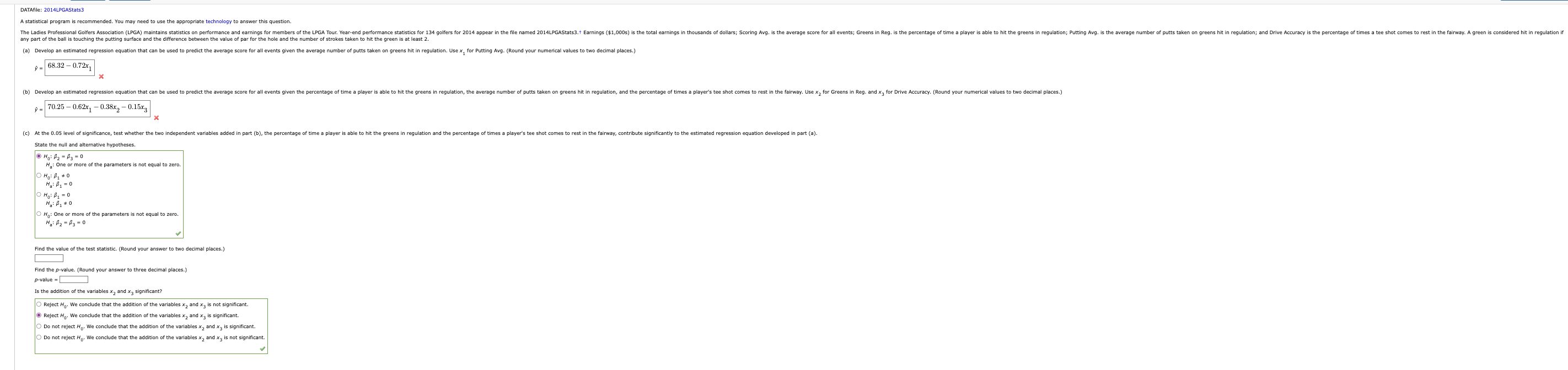
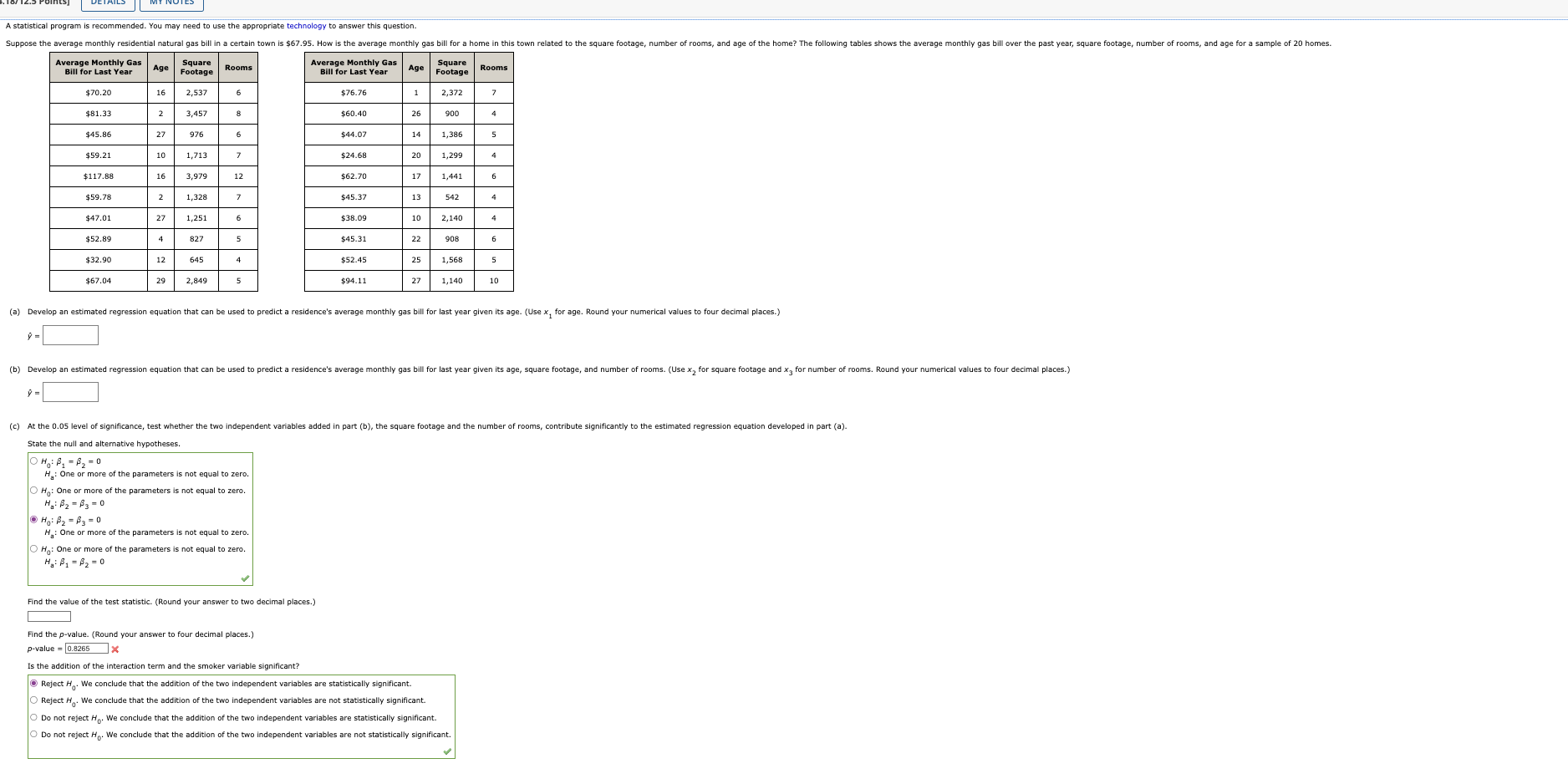
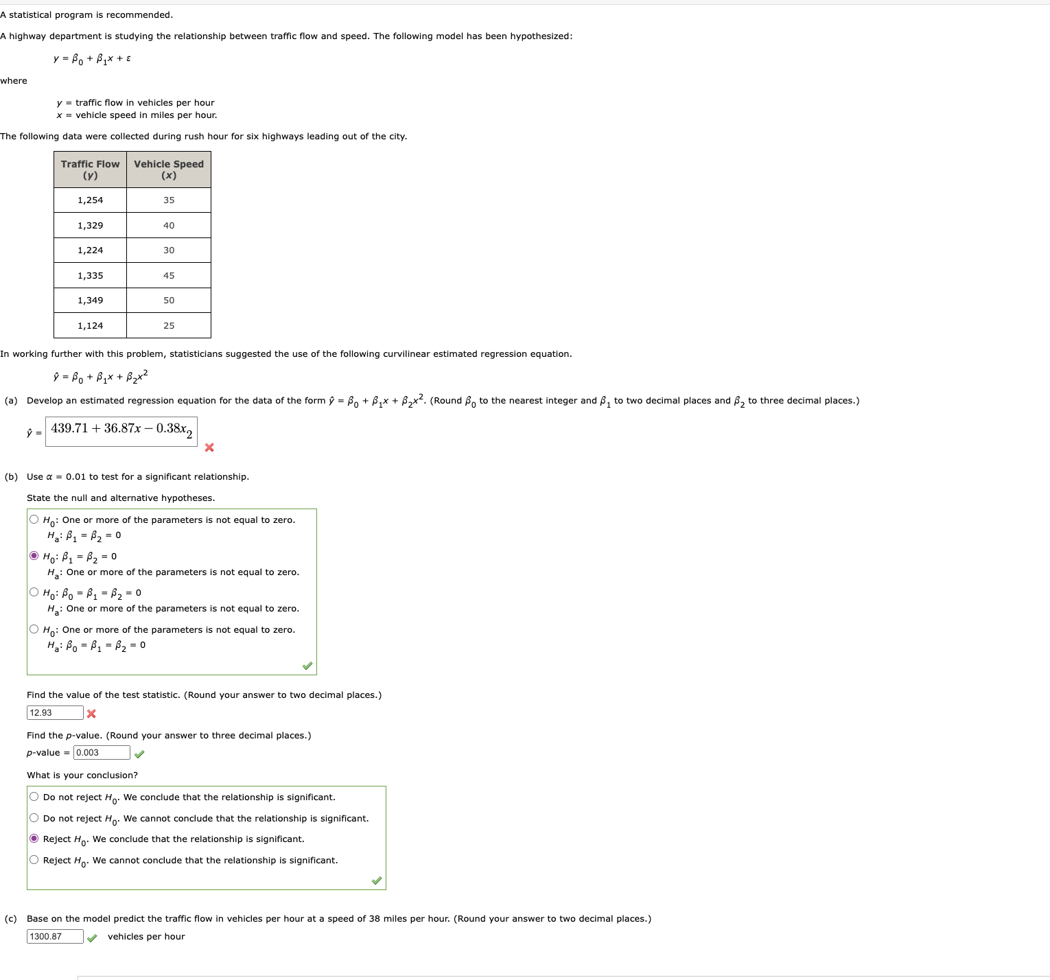
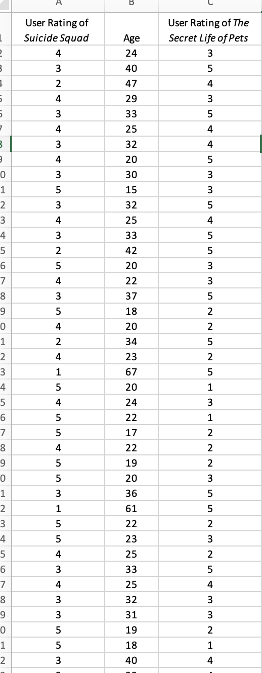
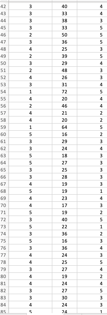
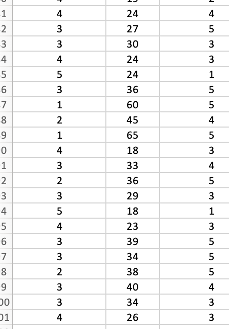
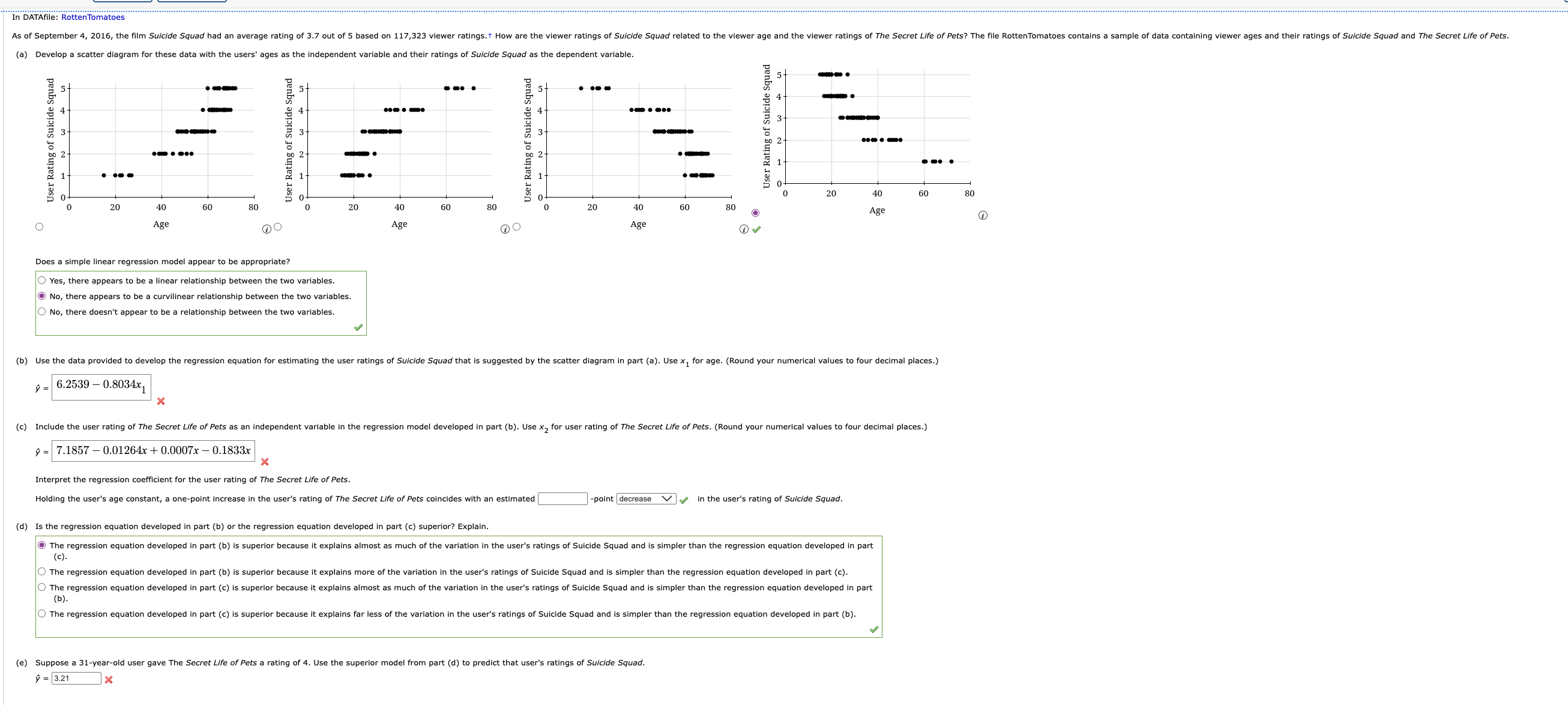
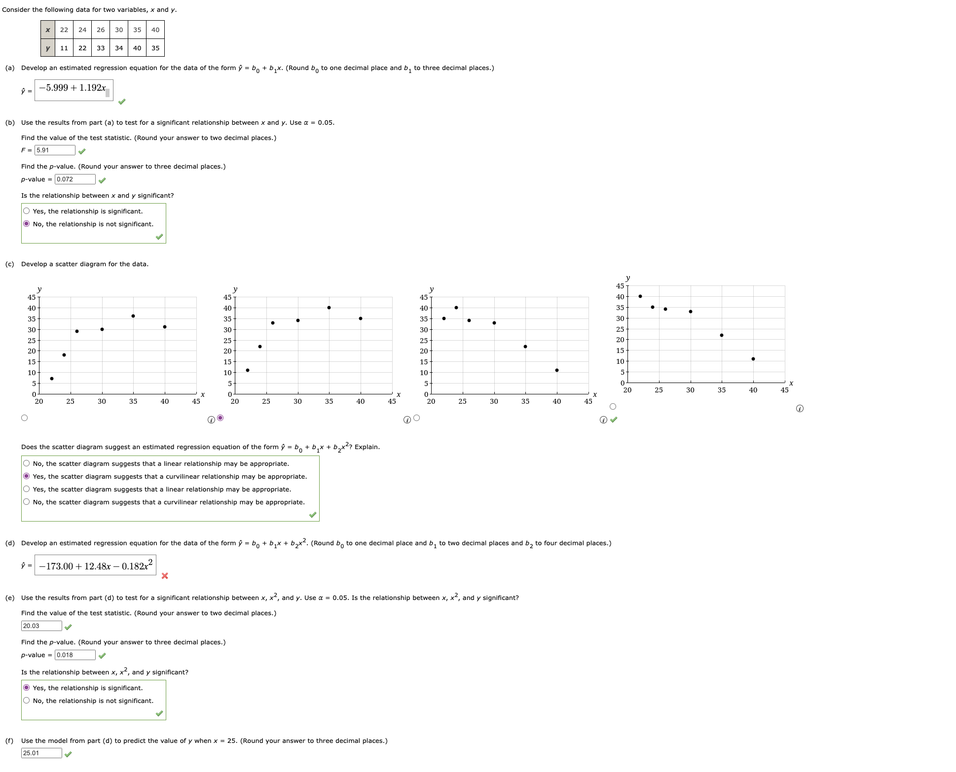
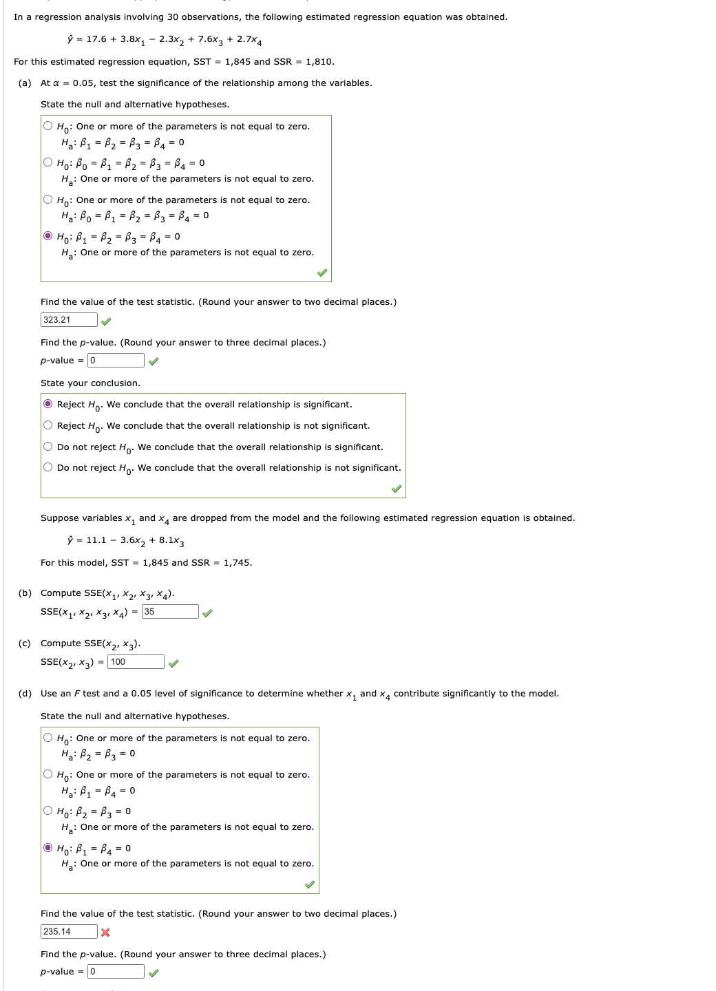
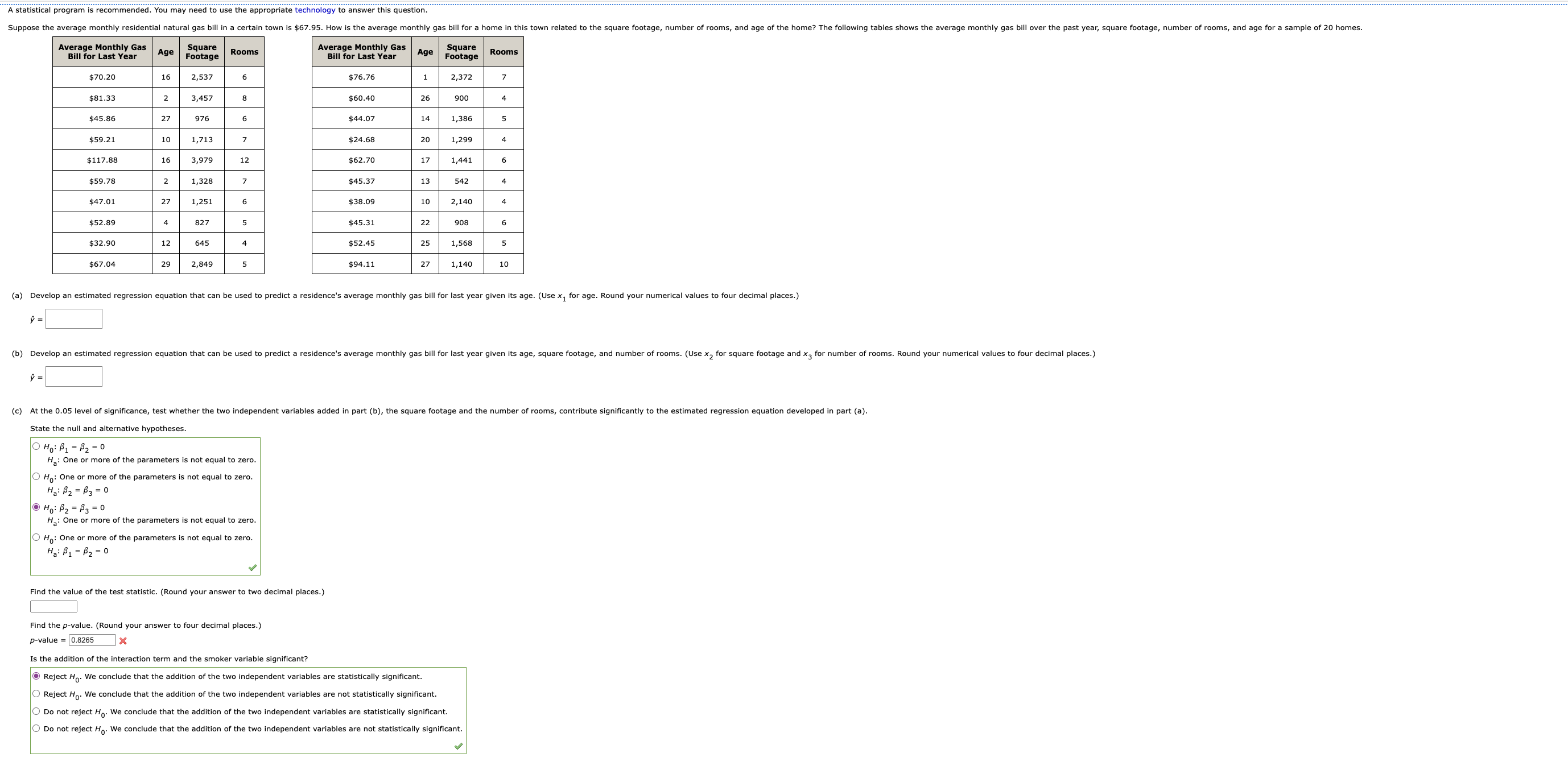
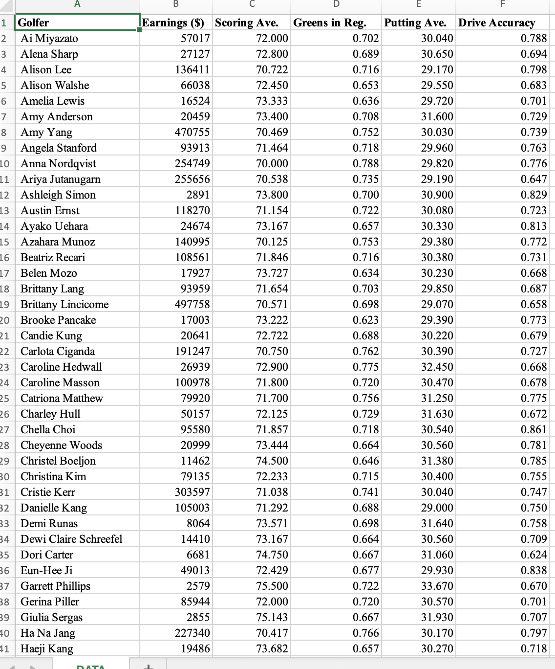
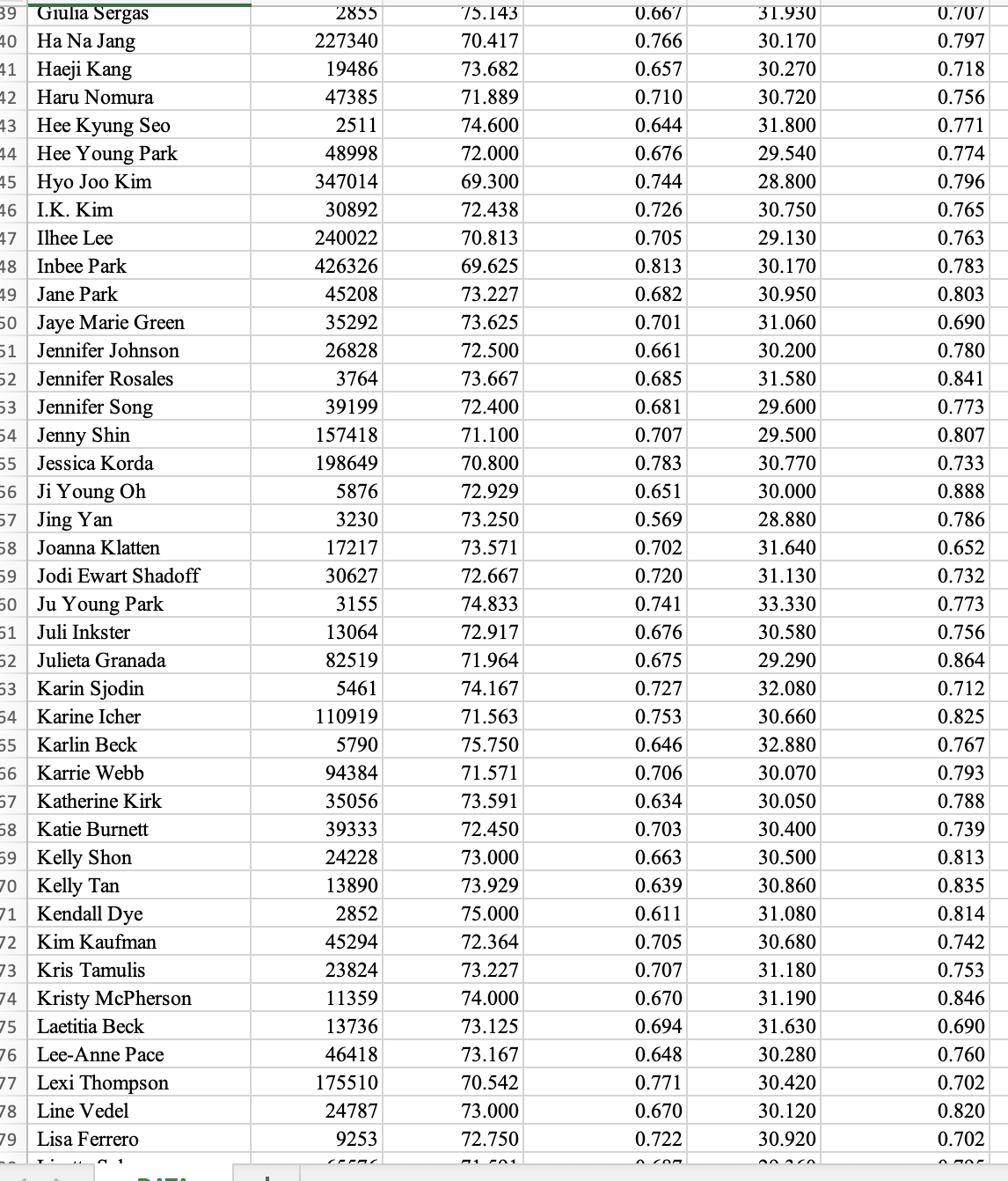
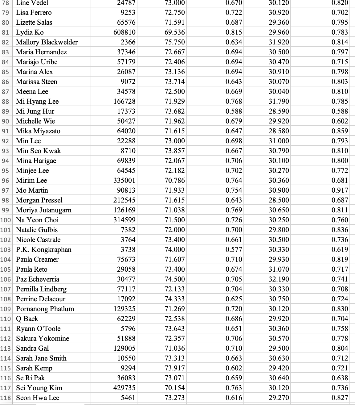
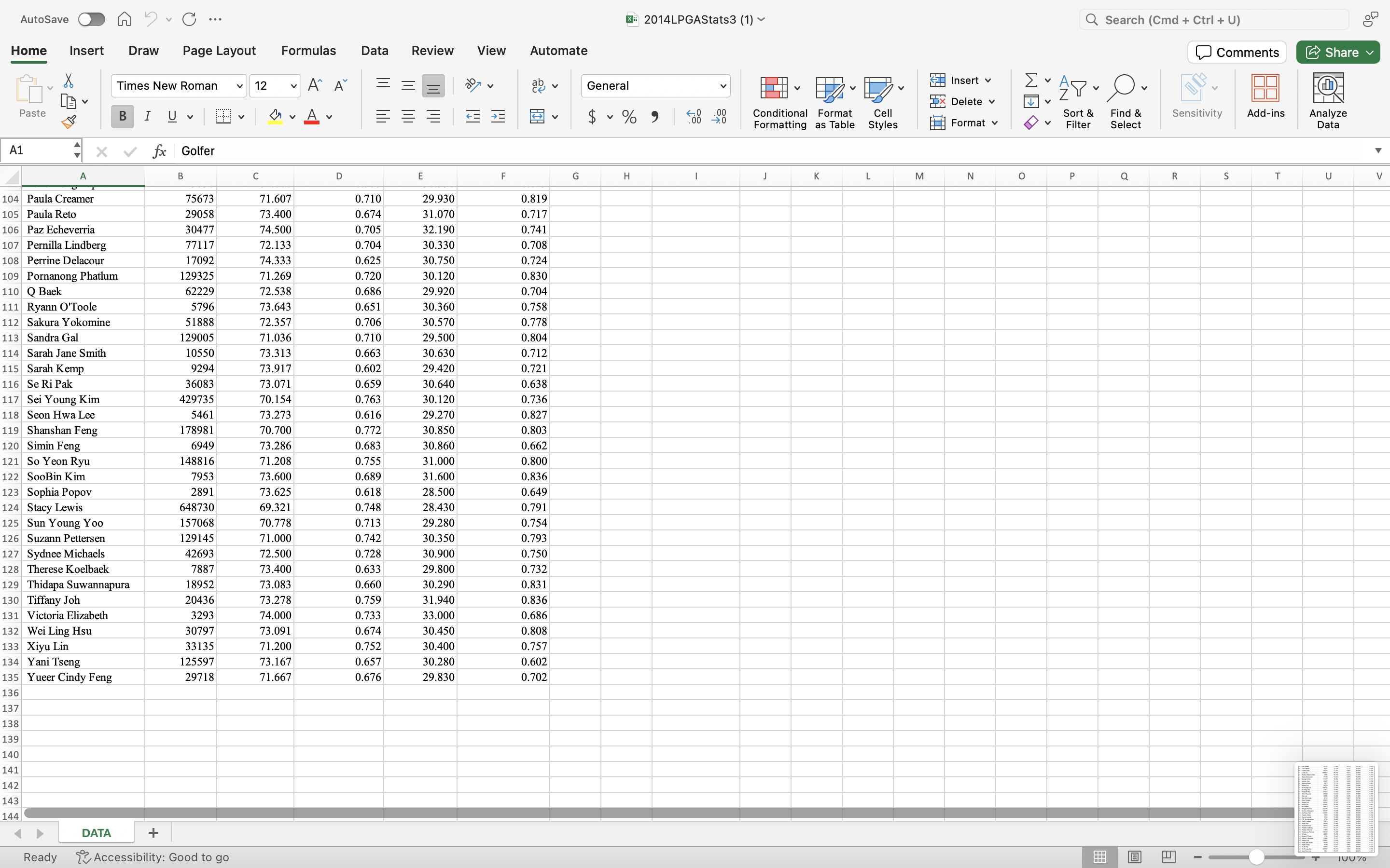
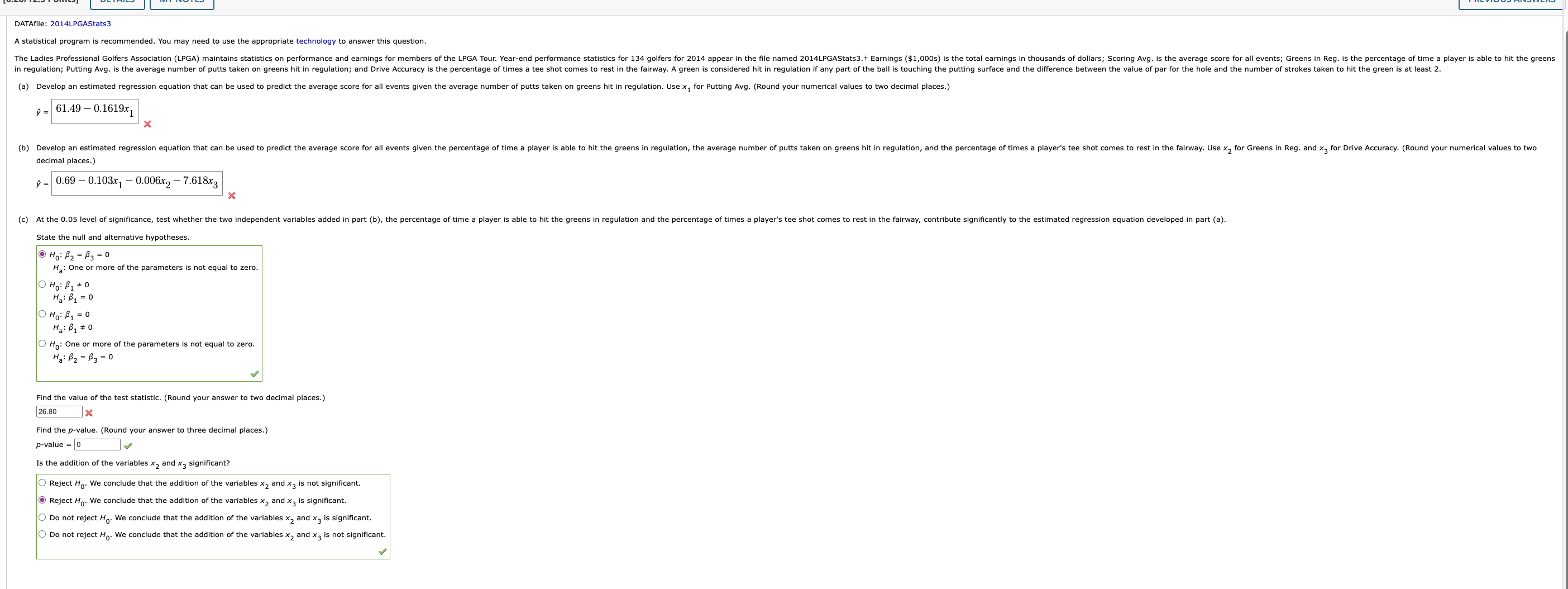
The owner of Showtime Movie Theaters, Inc., would like to predict weekly gross revenue as a function of advertising expenditures. Historical data for a sample of eight weeks follow. V:;er:ls(;y Television | Newspaper Revenue | Advertising | Advertising ($1,000s) | ($1/0005) | ($1,0005) 96 5.0 1.5 90 2.0 2.0 95 4.0 1.5 92 25 2.5 95 3.0 3.3 94 3.5 23 94 2.5 42 94 3.0 25 The owner then used multiple regression analysis to predict gross revenue (y), in thousands of dollars, as a function of television advertising (x, ), in thousands of dollars, and newspaper advertising (x;), in thousands of dollars. The estimated regression equation was J = 83.2 + 2.29x; + 1.30x,. (a) What is the gross revenue (in dollars) expected for a week when $2,500 is spent on television advertising (x1 = 2.5) and $2,500 is spent on newspaper advertising (x2 = 2.5)? (Round your answer to the nearest dollar.) $| (b) Provide a 95% confidence interval (in dollars) for the mean revenue of all weeks with the expenditures listed in part (a). (Round your answers to the nearest dollar.) s to$] | (c) Provide a 95% prediction interval (in dollars) for next week's revenue, assuming that the advertising expenditures will be allocated as in part (a). (Round your answers to the nearest dollar.) $ to$ J (5.02/6.66 Points] DETAILS MY NOTES The data below leage, age, and selling price for a sample of 33 sedans. Price Mileage | Ag 16,958 17,599 15,998 60,000 11,599 14,998 15,998 3 (a) Develop an estimated regression equation that predicts the selling mileage, *2 represent age, and y represent the selling price.] - 20227.84 - 0.03x1 - 752.19%2 (b) Is multicollinearity an issue for this model? Find the correlation b between the independent variables to answer this question.( Round your answer to two decimal places.) mileage is 0.65 . Since this is [ \\ 0.70, we conclude that multicollinearity [is not an issue. (c) Use the F test to de hiicance of the relationship. State the null and alternative hypotheses. H.: All the parameter M.: One or more of the beters is not equal to zero. He: One or more of the para H : A - D Calculate the test statistic. (Round your answer to two decimal places.) 138.22 % Calculate the p-value. (Round your answer to four decimal places.) p-value - 0 What is your conclusion at the 0.05 level of significance? . Reject H.- There is sufficient evidence to conclude that there is a significant relationship O Reject Ha- There is insufficient evidence to conclude that there is a significant relationship Do not reject Ho. There is sufficient evidence to conclude that there is a significant relationship. Do not reject Ho. There is insul relationship. e to conclude that there is a significant (d) use the t test to determine the significance of the independent variable mileage. State the null and alternative hypotheses. H . : A , - D Find the value of the test statistic for , . (Round your answer to two decimal places.) 4.76 * Find the p-value for #,. [Round your a decimal places.) povalue - 0 What is your conclusion at the 0.05 level of significance? . Reject H . There is sufficient evidence to conclude that mileage is a significant factor. O Reject H- There is insufficient evidence to conclude that mileage is a significant factor. Do not reject Ho. The Do not reject H. There is insufficient evi factor . e is a significant use the * test to determine the significance of the independent variable age. State the null and alternative hypotheses. OH: A2 - D HA, - D Find the value of the test statistic for #2. (Round your two decimal places.) -10.38 x Find the p-value for /2. (Round your answer to four decimal places.) p-value - 0 What is your conclusion at the 0.05 level of significance? * Reject Ho- There is sufficient evidence to conclude that age is a significant factor. is insufficient evidence to conclude that age is a significant factor. Do not reject H. There is sufficient evidence to conclude that age is a significant factor. Do not reject Hy. The factor. to conclude that age is a significantA statistical program is recommended. Consider the following data for two variables, x and y. * 22 24 26 30 35 40 11 22 33 34 40 35 (a) Develop an estimated regression equation for the data of the form " = by + bix. (Round by to one decimal place and b, to three decimal places.) (b) Use the results from part (a) to test for a significant relationship between x and y. Use a = 0.05. Find the value of the test statistic. (Round your answer to two decimal places.) Find the p-value. (Round your answer to three decimal places.) p-value =[ Is the relationship between x and y significant? O Yes, the relationship is significant No, the relationship is not significant. (c) Develop a scatter diagram for the data. 45 T 45 7 40 40 40 35 35 35 30 30 30 25 23 234 20 20 20 15 15/ 10+ ST 25 30 35 40 45 20 25 30 35 40 45 20 25 30 35 40 25 30 35 40 15 O Does the scatter diagram suggest an estimated regression equation of the form y = by + bix + b2x2? Explain. O No, the scatter diagram suggests near relationship may be appropriate. Yes, the scatter diagram sug r relationship may be appropriate. Yes, the scatter diagram suggests that a li ationship may be appropriate. No, the scatter diagram s relationship may be appropriate. (d) Develop an estimated regression equation for the data of the form ? = by + bj* + b2x2. (Round by to one decimal place and b, to two decimal places and b2 to four decimal places.) (e) Use the results from part (d) to test for a significant relationship between x, x2, and y. Use a = 0.05. Is the relationship between x, x2, and y significant? Find the value of the test statistic. (Round your answer to two decimal places.) Find the p-value. (Round your answer to three decimal places.) p-value = X Is the relationship between x, x", and y significant? Yes, the relationship is significant. No, the relationship is not significant. (f) Use the model from part (d) to predict the value of y when x = 25. (Round your answer to three decimal places.)A statistical program is recommended. A highway department is studying the relationship between traffic flow and speed. The following model has been hypothesized: = Fox+ where y = traffic flow in vehicles per hour x = vehicle speed in miles per hour. The following data were collected during rush hour for six highways leading out of the city. Traffic Flow | Vehicle Speed (v ) ( x ) 1,254 35 1,329 40 1,224 30 1,335 45 1,349 50 1,124 25 In working further with this problem, statisticians suggested the use of the following curvilinear estimated regression equation. (a) Develop an estimated regression equation for the data of the form = 8, + 8,* + 82*2. (Round #, to the nearest Integer and #, to two decimal places and #2 to three decimal places.) (b) Use a = 0.01 to test for a significant relationship. State the null and alternative hypotheses. O He: One or more of the parameters is not equal to zero. Ha : P1 = $2 = 0 OH:B, = $2 =0 He: One or more of the parameters is not equal to zero. O Ho: Bo = F1 = $2=0 He: One or more of the parameters is not equal to zero. O Ho: One or more of the parameters is not equal to zero. Hot Po = F1 = P2 = 0 Find the value of the test statistic. (Round your answer to two decimal places.) Find the p-value. (Round your answer to three decimal places.) -value = 0.003 What is your conclusion? O Do not reject Ho. We conclude that the relationship is significant. O Do not reject Ho. We cannot conclude that the relationship is significant. Reject Ho. We conclude that the relationship is significant. Reject Ho. We cannot conclude that the relationship is significant. (c) Base on the model predict the traffic flow in vehicles per hour at a speed of 38 miles per hour. (Round your answer to two decimal places.) is vehicles per hour Enter a number.In DATAfle; RottenTomatoe: As of September 4, 2016, the film Suicide Squad had an average rating of 3.7 out of 5 based on 117,323 viewer ratings. * How are the viewer ratings of Suicide Squad related to the viewer age and the viewer ratings of The Secret Life of Pets? The file RottenTomatoes contains a sample of data containing viewer ages and their ratings of Suicide Squad and The Secret Life of Pets. (2) Develop a scatter diagram for these data with the users' ages as the independent variable and thelr ratings of Suicide Squad as the dependent variable, 4 com o ame 4 oumoone 2 ouoose 2 2 o User Rating of S:lnde Squad | User Rating o suicide squad | User Ratingof Suicide squad | User Rating of Suicide Squad o 20 40 60 80 o 20 0 60 80 o 20 40 60 80 o Age o) Age Age Does a simple linear regression model appear to be appropriate? Yes, there appears to be a linear relationship between the two variables. No, there appears to be a curvilinear relationship between the two variables. No, there doesn't appear to be a relationship between the two variables. (b) Use the data provided to develop the regression equation for estimating the user ratings of Suicide Squad that is suggested by the scatter diagram In part (a). Use x, for age. (Round your numerical values to four decimal places.) fu L Ix (6) Include the user rating of The Secret Life of Pets as an Independent variable in the regression model developed in part (b). Use x, for user rating of The Secret Life of Pets. (Round your numerical values to four decimal places.) v x Interpret the regression coefficient for the user rating of The Secret Life of Pets. Holding the user's age constant, a one-point increase In the user's rating of The Secret Life of Pets coincides with an estimated ~point [decrease /] In the users rating of Suicide Squad. (d) T the regression equation developed in part (b) or the regression equation developed in part (c) superior? Explai The regression equation developed in part (b) is superior because it explains almost as much of the variation in the user's ratings of Suicide Squad and is simpler than the regression equation developed In part (. ) The regression equation developed in part (b) is superior because it explains more of the variation i the user's ratings of Suicide Squad and is simpler than the regression equation developed in part (c). O The regression equation developed In part (c) Is superior because It explains almost as much of the variation In the user's ratings of Suicide Squad and is simpler than the regression equation developed in part (). The regression equation developed in part (c) is superior because It explains far less of the variation in the user's ratings of Suicide Squad and Is simpler than the regression equation developed n part (b). v (e) Suppose a 31-year-old user gave The Secret Life of Pets a rating of 4. Use the superlor model from part (d) to predict that user's ratings of Suicide Squad. 7 x [11.25/12.5 Points] DETAILS MY NOTES You may need to use the appropriate technology to answer this question. In a regression analysis involving 30 observations, the following estimated regression equation was obtained. " = 17.6 + 3.8x, - 2.3x, + 7.6x,+ 2.7% For this estimated regression equation, SST = 1,845 and SSR = 1,810. (a) At a = 0.05, test the significance of the relationship among the variables. State the null and alternative hypotheses. O Ho: One or more of the parameters is not equal to zero. Ha: B1 = $2 = 83 = 84 =0 OHgi Bo = P1 = $2 = BJ = B. =0 H : One or more of the parameters is not equal to zero. Ha: One or more of the parameters is not equal to zero. H : Po = F1 = P2 = F] = B. =0 OH: B, = F, = 8, = =0 H : One or more of the parameters is not equal to zero. Find the value of the test statistic. (Round your answer to two decimal places.) 323.21 Find the p-value. (Round your answer to three decimal places.) p-value = 0 State your conclusion. Reject Ho. We conclude that the overall relationship is significant. O Reject Ho. We conclude that the overall relationship is not significant. O Do not reject Ho. We conclude that the overall relationship is significant. Do not reject Ho. We conclude that the overall relationship is not significant. Suppose variables x, and x, are dropped from the model and the following estimated regression equation is obtained. " = 11.1 - 3.6%2 + 8.1x] For this model, SST = 1,845 and SSR = 1,745. b) Compute SSE(X], X2, X3, *4). SSE(X ] , X2, *gr x) = 35 (c) Compute SSE(X2, x}). SSE(X2, X]) = 100 (d) Use an F test and a 0.05 level of significance to determine whether x, and x, contribute significantly to the model. State the null and alternative hypotheses. Hot One or more of the parameters is not equal to zero. He : B2 = 83 = 0 O Ho: One or more of the parameters is not equal to zero. Ha: P1 = FA =0 O Ho: B2 = F3 = 0 He : One or more of the parameters is not equal to zero. He : One or more of the parameters is not equal to zero. Find the value of the test statistic. (Round your answer to two decimal places.) ure pevalue. (Round your answer to three decimal places.) p-value = 0 State your conclusion. Do not reject H . We conclude that x, and x, contribute significantly to the model. Do not reject Ho. We conclude that x, and x, do not contribute significantly to the model. Reject Ho. We conclude that x, and x, do not contribute significantly to the model. Reject Ho. We conclude that x, and x, contribute significantly to the model.DATAfile: 2014LPGAStats3 statistical program is recommended. You may need to use the approp rofessional Golfers Association (LPGA) mainta any part of the ball is touching the putting surface and the mbers of the LPGA Tour. Year-er named 2014LPGAStats3.+ Earnings ($1,000s) is the tota (a) Develop an estimated regression equation that can be used lation. Use x, for Putting Avg. (Round your numer cimal places.) "= 68.32 - 0.72x1 (b) Develop an estimated regression equation that can be used to pre in the fairway. Use x2 for Greens in Reg. and x, for Drive Accuracy. (Round your numerical values to two decimal places.) 70.25 - 0.62x] - 0.38x2 - 0.1513 (c) At the 0.05 level of est whether the two in bed in part (a). State the null and alternative hypotheses. H: One or more of the parameters is not equal to zero. HOBO H.: B 1 0 Ho: One or more of the parameters is not equal to zero. H: P2 - 83 - 0 Find the value of the test statistic. (Round your answer to two decimal places.) Find the p-value. (Round your answer to three decimal places.) p-value = Is the addition of the variables x2 and *; significant? O Reject Ho. We conclude that the addition of the variables x2 and x} is not significant. Reject Ho. We conclude that the addition les x2 and X3 is significant. Do not reject Ho. We 3 Is significant. Do not reject Ho. We conclude that the addition of the variables x2 and x3 is not significant.A statistical program is recommended. You may need to use the appropriate technology to answer this question. Average Monthly Gas Bill for Last Year Age Square Suppose the average monthly residential natural gas bill in a certain town is $67.95. How is the average monthly gas bill for a home in this town related to the square footage, number of rooms, and age of the home? The following tables shows the average monthly gas bill over the past year, square footage, number of rooms, and age for a sample of 20 homes. Footage Rooms Average Monthly Gas Bill for Last Year Age Square Footage Rooms $70.20 16 2,537 $76.76 2,372 $81.33 3,457 60.40 26 900 $45.86 27 976 $44.07 14 1,386 $59.21 10 1,713 $24.68 20 1,299 $117.88 16 3,979 12 $62.70 17 1,441 6 59.78 2 1,328 $45.37 13 542 $47.01 27 1,251 $38.09 10 2,140 $52.89 827 :45.31 22 908 6 $32.90 12 645 :52.45 25 1,568 5 $67.04 29 2,84 $94.11 27 1,140 10 (a) Develop an estimated regression equation that can be used to predict a residence's average monthly gas bill for last year given its age. (Use x, for age. Round your numerical values to four decimal places.) D = (b) Develop an estimated regression equation that can be used to predict a residence's average monthly gas bill for last year given its age, square footage, and number of rooms. (Use x2 for square footage and x3 for number of rooms. Round your numerical values to four decimal places.) (c) At the 0.05 level of significance, test whether the two independent variables added in part (b), the square footage and the number of rooms, contribute significantly to the estimated regression equation developed in part (a). State the null and alternative hypotheses. OH : B = $2 =0 He : One or more of the parameters is not equal to zero. O Ho: One or more of the parameters is not equal to zero. Ha: P2 = $3 = 0 Ho: B2 = $3 = 0 He: One or more of the parameters is not equal to zero. O Ho: One or more of the parameters is not equal to zero. Ha: P1 = $2 = 0 Find the value of the test statistic. (Round your answer to two decimal places.) Find the p-value. (Round your answer to four decimal places.) -value = 0.8265 JX Is the addition of the interaction term and the smoker variable significant? Reject Ho. We conclude that the addition of the two inde lent variables are statistically significant. Reject Ho. We conclude that the addition of the two ind dent variables are not statistically significant. Do not reject Ho. We conclude that the addition of the two independent variables are statistically significant. O Do not reject Ho. We conclude that the addition of the two independent variables are not statistically significant.A statistical program is recommended A highway department is studying the relationship between traffic flow and speed. The following model has been hypothesized: y = BotBix+ where y = traffic flow in vehicles per hour