The person that answers this message, I would like to not only get the answer but also the formulas as well. I also need help with number 5 as well. I really don't know how to make the chart so if you can also show me the final result of this chart.

Thanks for all the help.

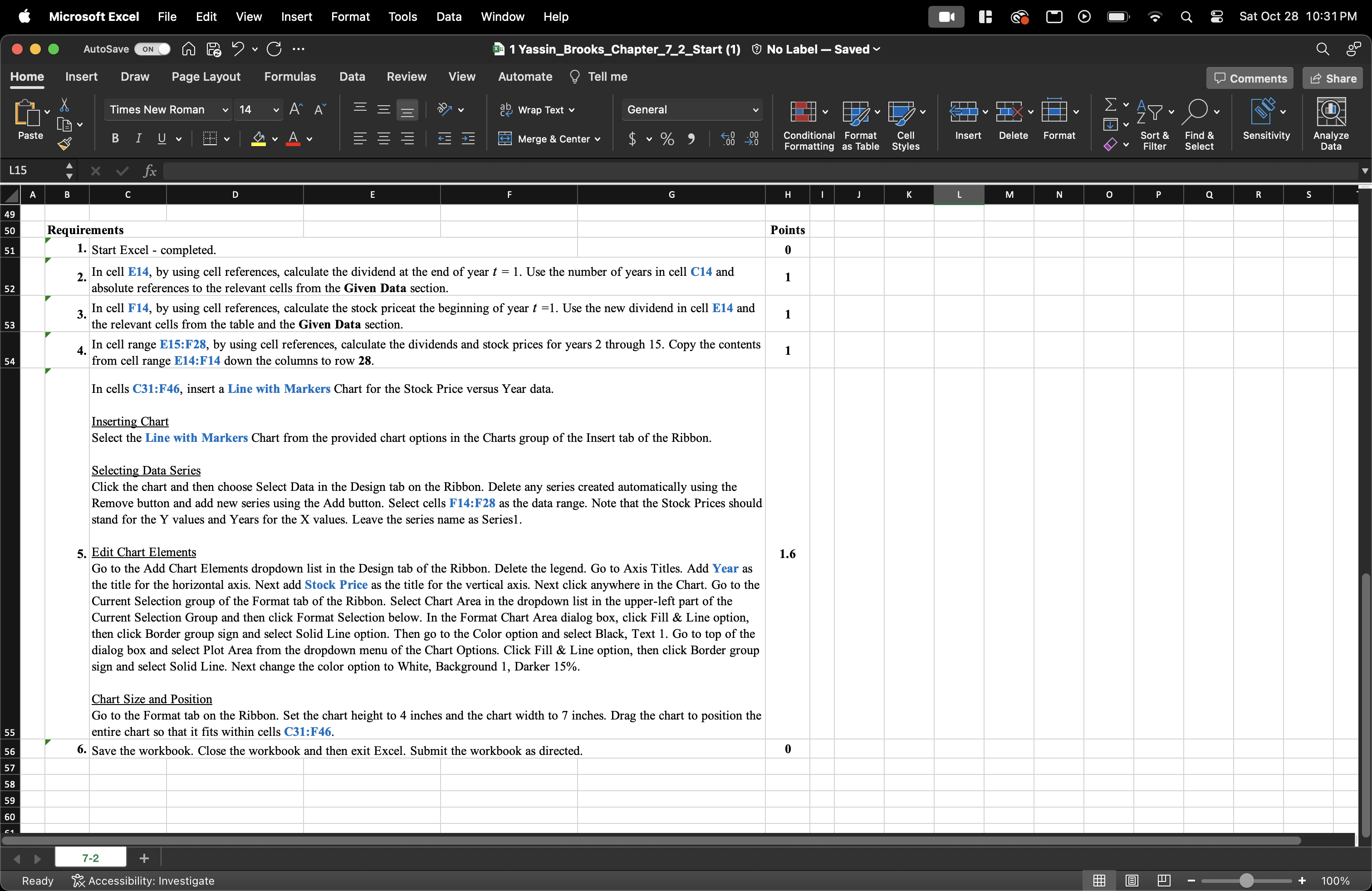
1. Start Excel - completed. 0 2. In cell E14, by using cell references, calculate the dividend at the end of year t=1. Use the number of years in cell C14 and absolute references to the relevant cells from the Given Data section. 3. In cell F14, by using cell references, calculate the stock priceat the beginning of year t=1. Use the new dividend in cell E14 and the relevant cells from the table and the Given Data section. 4. In cell range E15:F28, by using cell references, calculate the dividends and stock prices for years 2 through 15 . Copy the contents from cell range E14:F14 down the columns to row 28. In cells C31:F46, insert a Line with Markers Chart for the Stock Price versus Year data. Inserting Chart Select the Line with Markers Chart from the provided chart options in the Charts group of the Insert tab of the Ribbon. Selecting Data Series Click the chart and then choose Select Data in the Design tab on the Ribbon. Delete any series created automatically using the Remove button and add new series using the Add button. Select cells F14:F28 as the data range. Note that the Stock Prices should stand for the Y values and Years for the X values. Leave the series name as Series1. 5. Edit Chart Elements Go to the Add Chart Elements dropdown list in the Design tab of the Ribbon. Delete the legend. Go to Axis Titles. Add Year as the title for the horizontal axis. Next add Stock Price as the title for the vertical axis. Next click anywhere in the Chart. Go to the Current Selection group of the Format tab of the Ribbon. Select Chart Area in the dropdown list in the upper-left part of the Current Selection Group and then click Format Selection below. In the Format Chart Area dialog box, click Fill \& Line option, then click Border group sign and select Solid Line option. Then go to the Color option and select Black, Text 1. Go to top of the dialog box and select Plot Area from the dropdown menu of the Chart Options. Click Fill \& Line option, then click Border group sign and select Solid Line. Next change the color option to White, Background 1, Darker 15\%. Chart Size and Position Go to the Format tab on the Ribbon. Set the chart height to 4 inches and the chart width to 7 inches. Drag the chart to position the entire chart so that it fits within cells C31:F46. 6. Save the workbook. Close the workbook and then exit Excel. Submit the workbook as directed. 1.6