The topic is on Capital Budgeting. Introductory to finance.

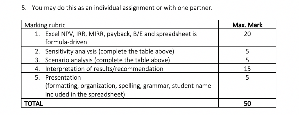
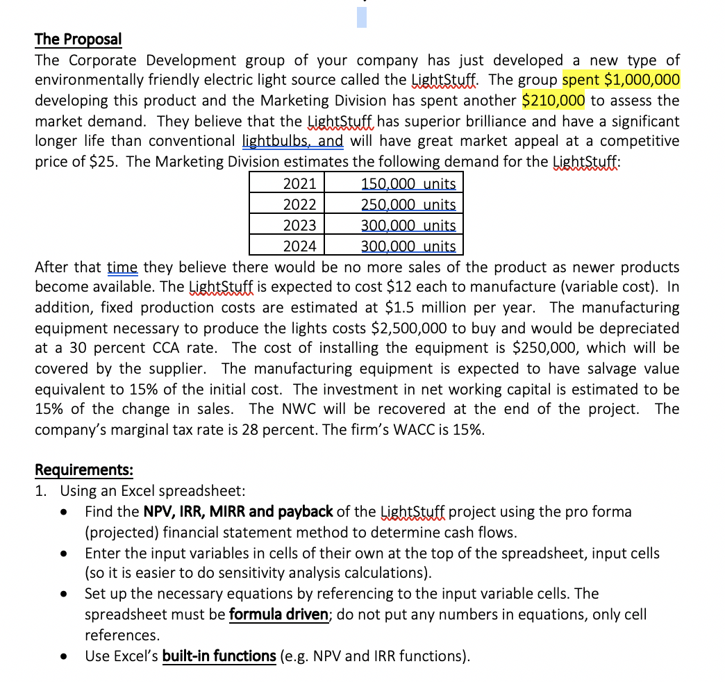
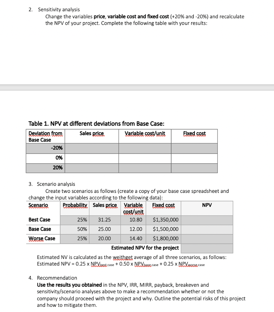
5. You may do this as an individual assignment or with one partner. Max. Mark 20 5 5 Marking rubric 1. Excel NPV, IRR, MIRR, payback, B/E and spreadsheet is formula-driven 2. Sensitivity analysis (complete the table above) 3. Scenario analysis (complete the table above) 4. Interpretation of results/recommendation 5. Presentation (formatting, organization, spelling, grammar, student name included in the spreadsheet) TOTAL 15 50 The Proposal The Corporate Development group of your company has just developed a new type of environmentally friendly electric light source called the LightStuff. The group spent $1,000,000 developing this product and the Marketing Division has spent another $210,000 to assess the market demand. They believe that the LightStuff has superior brilliance and have a significant longer life than conventional lightbulbs, and will have great market appeal at a competitive price of $25. The Marketing Division estimates the following demand for the LightStuff: 2021 150.000 units 2022 250.000 units 2023 300.000 units 2024 300.000 units After that time they believe there would be no more sales of the product as newer products become available. The LightStuff is expected to cost $12 each to manufacture (variable cost). In addition, fixed production costs are estimated at $1.5 million per year. The manufacturing equipment necessary to produce the lights costs $2,500,000 to buy and would be depreciated at a 30 percent CCA rate. The cost of installing the equipment is $250,000, which will be covered by the supplier. The manufacturing equipment is expected to have salvage value equivalent to 15% of the initial cost. The investment in net working capital is estimated to be 15% of the change in sales. The NWC will be recovered at the end of the project. The company's marginal tax rate is 28 percent. The firm's WACC is 15%. Requirements: 1. Using an Excel spreadsheet: Find the NPV, IRR, MIRR and payback of the LightStuff project using the pro forma (projected) financial statement method to determine cash flows. Enter the input variables in cells of their own at the top of the spreadsheet, input cells (so it is easier to do sensitivity analysis calculations). Set up the necessary equations by referencing to the input variable cells. The spreadsheet must be formula driven; do not put any numbers in equations, only cell references. Use Excel's built-in functions (e.g. NPV and IRR functions). 2. Sensitivity analysis Change the variables price, variable cost and fixed cost (+20% and -20%) and recalculate the NPV of your project. Complete the following table with your results: Table 1. NPV at different deviations from Base Case: Deviation from Sales price Variable cost/unit Base Case -20% Fixed cost 0% 20% 3. Scenario analysis Create two scenarios as follows (create a copy of your base case spreadsheet and change the input variables according to the following data): Scenario Probability Sales price Variable Fixed cost NPV cost/unit Best Case 25% 31.25 10.80 $1,350,000 Base Case 25.00 12.00 $1,500,000 Worse Case 25% 20.00 14.40 $1,800,000 Estimated NPV for the project Estimated NV is calculated as the weithget average of all three scenarios, as follows: Estimated NPV = 0.25 x NPVhest case + 0.50 x NPV base, case + 0.25 x NPV worse case 50% 4. Recommendation Use the results you obtained in the NPV, IRR, MIRR, payback, breakeven and sensitivity/scenario analyses above to make a recommendation whether or not the company should proceed with the project and why. Outline the potential risks of this project and how to mitigate them. 5. You may do this as an individual assignment or with one partner. Max. Mark 20 5 5 Marking rubric 1. Excel NPV, IRR, MIRR, payback, B/E and spreadsheet is formula-driven 2. Sensitivity analysis (complete the table above) 3. Scenario analysis (complete the table above) 4. Interpretation of results/recommendation 5. Presentation (formatting, organization, spelling, grammar, student name included in the spreadsheet) TOTAL 15 50 The Proposal The Corporate Development group of your company has just developed a new type of environmentally friendly electric light source called the LightStuff. The group spent $1,000,000 developing this product and the Marketing Division has spent another $210,000 to assess the market demand. They believe that the LightStuff has superior brilliance and have a significant longer life than conventional lightbulbs, and will have great market appeal at a competitive price of $25. The Marketing Division estimates the following demand for the LightStuff: 2021 150.000 units 2022 250.000 units 2023 300.000 units 2024 300.000 units After that time they believe there would be no more sales of the product as newer products become available. The LightStuff is expected to cost $12 each to manufacture (variable cost). In addition, fixed production costs are estimated at $1.5 million per year. The manufacturing equipment necessary to produce the lights costs $2,500,000 to buy and would be depreciated at a 30 percent CCA rate. The cost of installing the equipment is $250,000, which will be covered by the supplier. The manufacturing equipment is expected to have salvage value equivalent to 15% of the initial cost. The investment in net working capital is estimated to be 15% of the change in sales. The NWC will be recovered at the end of the project. The company's marginal tax rate is 28 percent. The firm's WACC is 15%. Requirements: 1. Using an Excel spreadsheet: Find the NPV, IRR, MIRR and payback of the LightStuff project using the pro forma (projected) financial statement method to determine cash flows. Enter the input variables in cells of their own at the top of the spreadsheet, input cells (so it is easier to do sensitivity analysis calculations). Set up the necessary equations by referencing to the input variable cells. The spreadsheet must be formula driven; do not put any numbers in equations, only cell references. Use Excel's built-in functions (e.g. NPV and IRR functions). 2. Sensitivity analysis Change the variables price, variable cost and fixed cost (+20% and -20%) and recalculate the NPV of your project. Complete the following table with your results: Table 1. NPV at different deviations from Base Case: Deviation from Sales price Variable cost/unit Base Case -20% Fixed cost 0% 20% 3. Scenario analysis Create two scenarios as follows (create a copy of your base case spreadsheet and change the input variables according to the following data): Scenario Probability Sales price Variable Fixed cost NPV cost/unit Best Case 25% 31.25 10.80 $1,350,000 Base Case 25.00 12.00 $1,500,000 Worse Case 25% 20.00 14.40 $1,800,000 Estimated NPV for the project Estimated NV is calculated as the weithget average of all three scenarios, as follows: Estimated NPV = 0.25 x NPVhest case + 0.50 x NPV base, case + 0.25 x NPV worse case 50% 4. Recommendation Use the results you obtained in the NPV, IRR, MIRR, payback, breakeven and sensitivity/scenario analyses above to make a recommendation whether or not the company should proceed with the project and why. Outline the potential risks of this project and how to mitigate them