There is the code.

from PIL import Image import numpy as np import matplotlib.pyplot as plt from scipy import signal import math from demos.demo02 import harris

def plot_1D_gaussian(mu, variance, color='orange', x_limit=3): sigma = math.sqrt(variance) # get 100 'x' values between mu - x_limit * sigma and mu + x_limit * sigma x = np.linspace(mu - x_limit * sigma, mu + x_limit * sigma, 100) y = np.exp(-np.power(x - mu, 2.) / (2 * variance))/(np.sqrt(2 * np.pi * variance)) plt.plot(x, y, color)

def plot_2D_surface(matrix_2d): kernel_size = matrix_2d.shape X, Y = np.meshgrid(np.linspace(-kernel_size[0] // 2, kernel_size[0] // 2, kernel_size[0]), np.linspace(-kernel_size[1] // 2, kernel_size[1] // 2, kernel_size[1])) plt.figure() ax = plt.axes(projection='3d') ax.plot_surface(X, Y, matrix_2d)

def gaussian_2D_kernel(size=5, sigma=3.0): # get x, y coordinates using np.meshgrid function x, y = np.meshgrid(np.linspace(-1, 1, size), np.linspace(-1, 1, size)) # YOUR CODES #1 6 points # Step 1: Compute a 2D gaussian kernel and store it in kernel # Step 2: Compute the normalized kernel and store it in kernel_norm # Hint: the sum of the numbers in the kernel is 1.0 kernel kernel_norm print("2D Gaussian-like array:") print(kernel_norm) return kernel_norm

def main(): path = '../../data/empire.jpg' im = np.array(Image.open(path).convert('L'))

""" Part 1 Gaussian """ kernel_size = 11 # odd number # get gaussian kernel kernel = gaussian_2D_kernel(size=kernel_size, sigma=2.0)

# Apply Gaussian Blurring to the image using convolution im_blurring = signal.convolve2d(im, kernel, boundary='symm', mode='same')

""" Part 2 Harris Corner Detector """ im_harris = harris.compute_harris_response(im) # Get harris points by setting min_dist = 30 and threshold = 0.01 # Store the results in a numpy array filtered_cords # YOUR CODES #2 2 points filtered_cords

""" Part 3 Homography """ # The corners of a rectangle are located at (-0.6, -0.3), (0.6, -0.3), (0.6, 0.3) and (-0.6, 0.3) # Use a two-row numpy array to store the coordinates # YOUR CODES #3 3 points points

# Use np.vstack to obtain the homogeneous coordinates # YOUR CODES #4 3 points points_norm

# Define two affine transformation matrices. # Obtain the new coordinates and store them in points_norm_s and points_norm_sr # YOUR CODES #5 9 points # Scaling

points_norm_s # Rotation (about the origin)

points_norm_sr

# Plot the Kernel plot_2D_surface(kernel)

# construct a second figure plt.figure() plt.gray() # use subplot to display the images using a 2 by 2 setting plt.subplot(2, 2, 1) plot_1D_gaussian(0, 0.2, 'b') # YOUR CODES #6 4 points

plt.subplot(2, 2, 2) # YOUR CODES #7 3 points # On the blurred image, show 10 strongest harris points using cyan marks

plt.subplot(2, 2, 3) plt.axis('equal') plt.plot(points_norm[0], points_norm[1], 'g')

plt.subplot(2, 2, 4) plt.axis('equal') plt.plot(points_norm_s[0], points_norm_s[1], 'b') plt.plot(points_norm_sr[0], points_norm_sr[1], 'r') plt.show()

if __name__ == '__main__': main()

YOUR ONLY NEED FINISH THE CODE 3 AND CODE 4

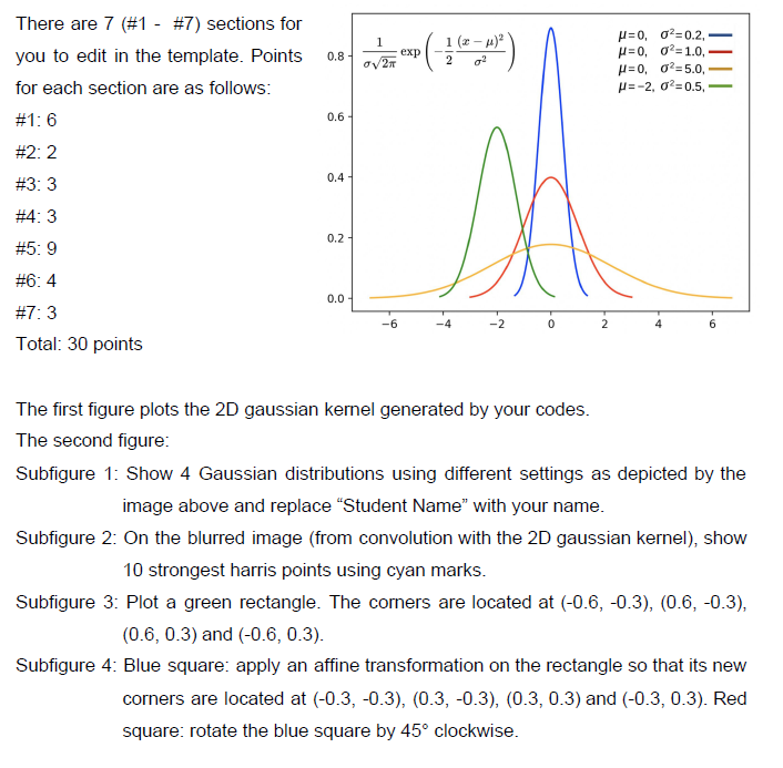
1 1 (2-4) g? 0.8 exp 2 There are 7 (#1 - #7) sections for you to edit in the template. Points for each section are as follows: #1: 6 027 =0,02=0.2, =0,02=1.0, p=0,02=5.0 = -2, 02-0.5, 0.6 #2:2 0.4 #3:3 #4:3 Da 0.2 #5: 9 #6:4 0.0 -6 -2 0 2 6 #7: 3 Total: 30 points The first figure plots the 2D gaussian kernel generated by your codes. The second figure: Subfigure 1: Show 4 Gaussian distributions using different settings as depicted by the image above and replace Student Name" with your name. Subfigure 2: On the blurred image (from convolution with the 2D gaussian kernel), show 10 strongest harris points using cyan marks. Subfigure 3. Plot a green rectangle. The corners are located at (-0.6, -0.3), (0.6, -0.3), (0.6, 0.3) and (-0.6, 0.3). Subfigure 4: Blue square: apply an affine transformation on the rectangle so that its new corners are located at (-0.3, -0.3), (0.3,-0.3), (0.3, 0.3) and (-0.3, 0.3). Red square: rotate the blue square by 45 clockwise. 1 1 (2-4) g? 0.8 exp 2 There are 7 (#1 - #7) sections for you to edit in the template. Points for each section are as follows: #1: 6 027 =0,02=0.2, =0,02=1.0, p=0,02=5.0 = -2, 02-0.5, 0.6 #2:2 0.4 #3:3 #4:3 Da 0.2 #5: 9 #6:4 0.0 -6 -2 0 2 6 #7: 3 Total: 30 points The first figure plots the 2D gaussian kernel generated by your codes. The second figure: Subfigure 1: Show 4 Gaussian distributions using different settings as depicted by the image above and replace Student Name" with your name. Subfigure 2: On the blurred image (from convolution with the 2D gaussian kernel), show 10 strongest harris points using cyan marks. Subfigure 3. Plot a green rectangle. The corners are located at (-0.6, -0.3), (0.6, -0.3), (0.6, 0.3) and (-0.6, 0.3). Subfigure 4: Blue square: apply an affine transformation on the rectangle so that its new corners are located at (-0.3, -0.3), (0.3,-0.3), (0.3, 0.3) and (-0.3, 0.3). Red square: rotate the blue square by 45 clockwise